Faking a Logarithmic Bitcoin Price Growth Model

Neither the dog nor the road - just a drunkard.

Short review

This article explores the question of whetheris there any relationship betweentime and price of bitcoin. We will check the proposed [here: 1, 2, 3] double logarithmic model for statistical reliability using the least squares method, as well as for stationarity with respect to each variable and potential false dependencies, using the Angle – Granger method for cointegration analysis. The results of all tests, except one, refute the hypothesis that time can be an important predictor of the price of bitcoin.

Introduction

Model log price ~ log time (aka logarithmic growth model) was proposed by several authors [1, 2, 3] to explain a significant part of Bitcoin price movements in the past and, as a result, to predict future prices.

The scientific method is difficult for most people to understand.This can lead to conclusions that do not reflect personal beliefs.In order to understand this method, it is necessary to understand and accept its fundamental idea:make mistakes normally.

According to the great philosopher of science KarlPopper, testing a hypothesis for its fallacy is the only reliable way to add weight to the argument that it is true. If rigorous multiple tests cannot prove that the hypothesis is erroneous, then with each such test the likelihood that it is true increases. This concept is called the falsifiability (or potential disproof) of the hypothesis. In this article, I will try to falsify the model of the logarithmic increase in the price of bitcoin in the form as it was formulated in the three sources indicated above: 1, 2, 3.

Notes:

• For all analyzes, Stata 14 software was used.
• The article does not contain financial recommendations.

Problem definition

In order to falsify a hypothesis, you first need to establish exactly what it consists of:

Zero Hypothesis (H0): The price of Bitcoin is a function of the number of days that Bitcoin has existed.

Alternative Hypothesis (H1): Bitcoin Pricenotis a function of the number of days that Bitcoin exists.

The authors of the above sources decided to checkH0 by selecting the regression of the usual least squares (OLS) to the natural logarithm of the price of Bitcoin and the natural logarithm of the number of days of the existence of Bitcoin. None of the authors gave any concomitant diagnostics, or any specific reason for the logarithmic transformation of both variables. The model did not take into account the possibility of establishing a false dependence due to non-stationarity, the possibility of interaction, or other distorting factors.

Method

In today's article, we will look at this model,we will diagnose normal regression and determine whether the transformation of the logarithm was necessary or appropriate (or both), and also examine possible distorting factors (confounders), interactions and the sensitivity of the model to distortions.

Another issue we are investigating isnon-stationary problem. Stationarity (invariance in time) is a prerequisite for most statistical models. This refers to the idea that if a trend relative to time is absent in average values ​​(or variance), then it is absent at any moment in time.

In addition to stationarity analysis, we are also exploring the possibility of cointegration.

Legend

Traditionally, the calculated value of a statistical parameter is denoted by a "cap" above the symbol.Calculated valueβ= [βMatrix 2×2 will be represented as [r1c1, r1c2, r2c1, r2c2], and so on.To denote indexed elements, we will use the @ symbol – for example, for the 10th position in vector X, X is usually used with a subscript of 10.Instead, we'll be writing X@10.

Ordinary least squares

Regular least squares regression is a method of finding a linear relationship between two or more variables.

First, let's define a linear model as some function X, which is equal to Y with some error.

Y = βX + ε

where Y is the dependent variable, X is the independent variable,εis the magnitude of the error, andβ– multiplierX. The job of OLS is to output the valueβso as to minimizeε.

In order to derive a reliable calculated value [β], it is necessary to observe some basic conditions (known as conditions to the Gauss – Markov Theorem):

1. The presence of a linear relationship between dependent and independent variables
2. Homoskedasticity (i.e. constant dispersion) of errors
3. The average value of the error distribution is usually zero
4. Lack of autocorrelation of errors (that is, they do not correlate with the sequence of errors taken with a time shift)

Linearity

We start by looking at the relationship between the price and the number of days that has not been converted to a dispersion diagram (Coinmetrics data).

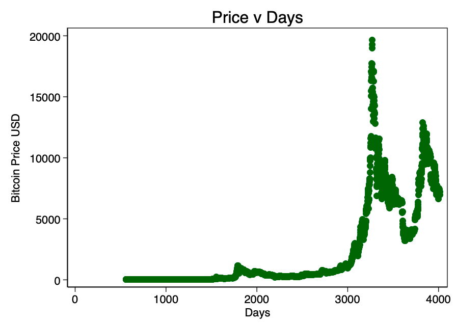
Fig. 1 - The ratio of the price to the number of days. The data is scattered too wide to determine the linearity visually.

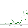
Figure 1 clearly shows sufficient reason fortaking the logarithm of the price: the range of values ​​is too large. When taking the logarithm of the price (but not the number of days) and re-plotting the chart, we get a familiar pattern (Figure 2).

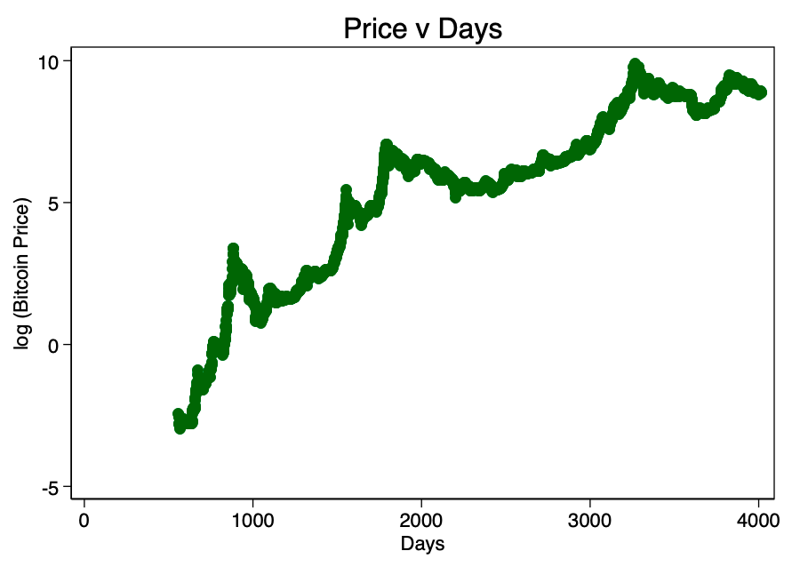
Fig. 2 - The ratio of the logarithm of the price to the number of days. There is a distinct logarithmic pattern.

Taking the logarithm of the number of days and plotting a chart already with it, we get an obvious linear pattern identified by the authors of our three sources (see the beginning of the article) in Figure 3.

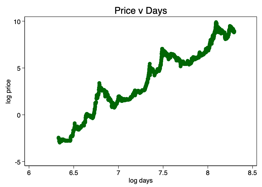
Fig. 3 - an obvious linear relationship arises.

This confirms the correct choice of the double logarithm as the only option that results in a well-visible linear relationship.

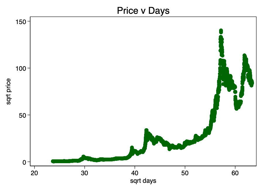
Fig. 4 - square root transformations give not much better result than untransformed data

Thus, preliminary analysis does not refute H0.

The results of the double logarithmic regression are shown in Figure 5 below, where [β] =5.8.

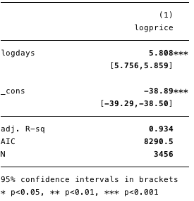
Figure 5 - Results for a double logarithmic regression.

Using this model, we can now determine the residuals [ε] and calculated values ​​[Y], and also check compliance with other conditions.

Homoskedasticity

If the condition of constant dispersion inthe magnitude of the error (i.e., homoscedasticity), the error for each value of the predicted cost fluctuates randomly around zero. Therefore, the graph of the ratio of residual value to estimated value (Fig. 6) is a simple but effective way to graphically verify the fulfillment of this condition. In Figure 6, we see a clearly defined pattern rather than random scattering, indicating that the variance in the magnitude of the error is inconsistent (i.e., heteroscedasticity).

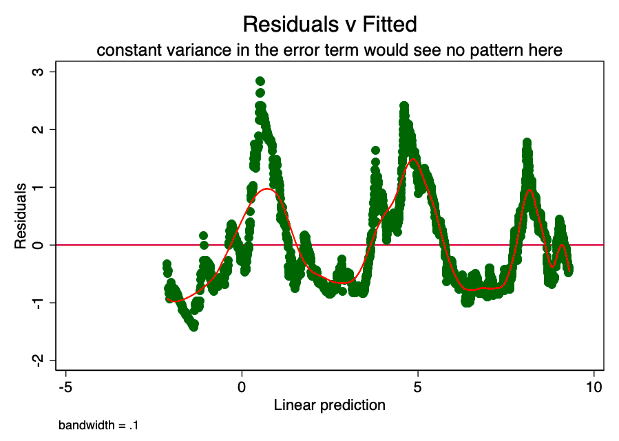
Fig. 6 (a) is a graph of the ratio of residual value to estimated. The presence of a pattern here indicates a probable problem.

The consequence of such heteroscedasticity is a larger dispersion and, accordingly, a lower accuracy of the calculated values ​​of the coefficients [β]. In addition, it leads to greater than it should be, the significance of p-values, since the OLS method does not reveal increased variance. Therefore, to calculate t- and F-values, we use an underestimated dispersion value, leading to a higher significance. It also affects the 95% confidence interval for [β], which is also a function of variance (through standard error).

The results of the Broch - Godfrey autocorrelation test also indicate the presence of this problem.

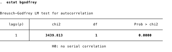
Fig. 6 (b) - Autocorrelation in residues

It’s usually worth stopping at this stage andclarify the model. However, given that we know the effect of these problems, it will be relatively safe to continue with a regression understanding that these problems exist. Ways to deal with them (at least in their lightest form) exist - for example, taking bootstrap samples or a robust dispersion estimate.

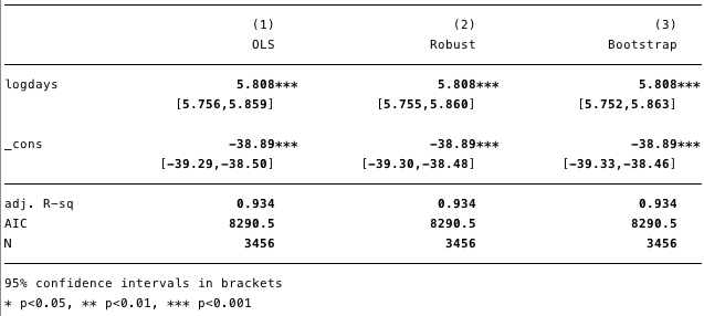
Fig. 7 - The effect of heteroskedasticity in various evaluations.

As can be seen in Figure 7, despite a smallan increase in variance (see extended confidence interval), by and large, the present heteroskedasticity in reality does not have too much harmful effect.

Normal error distribution

Satisfaction of the condition that the error indistributed with an average value of zero is not as important as satisfying the conditions of linearity or homoskedasticity. If the residuals do not correspond to the normal distribution but are not distorted, confidence intervals will be overly optimistic. If the residuals are distorted, then the final result may be distorted. As can be seen from Figures 8 and 9, the residues are highly distorted. The test for normality by the Shapiro-Wilk criterion gives a p-value equal to 0. They do not correspond to the normal curve sufficiently so that confidence intervals are not affected.

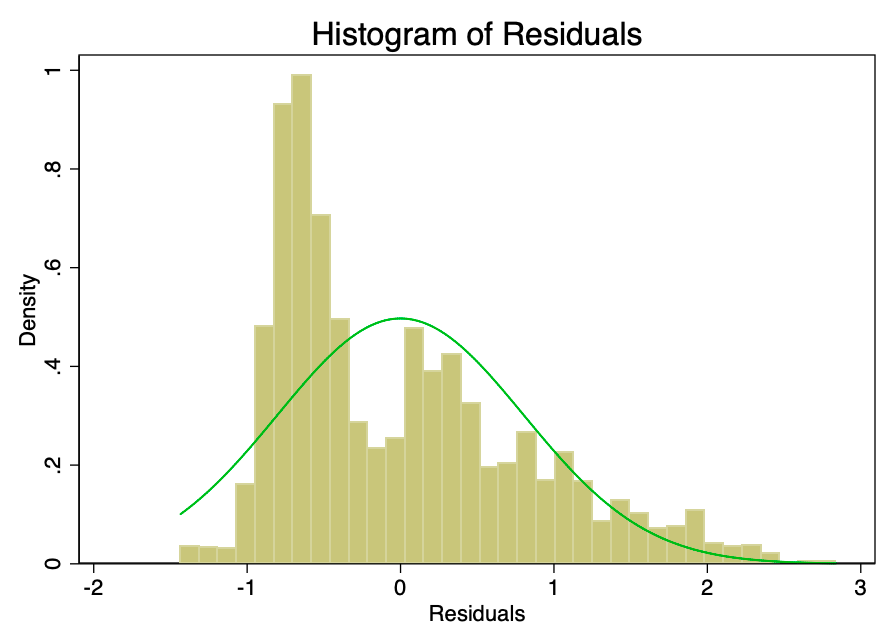
Fig. 8 - Histogram of the error with the (green) normal distribution curve superimposed on it. The error should be normal, but it is not.

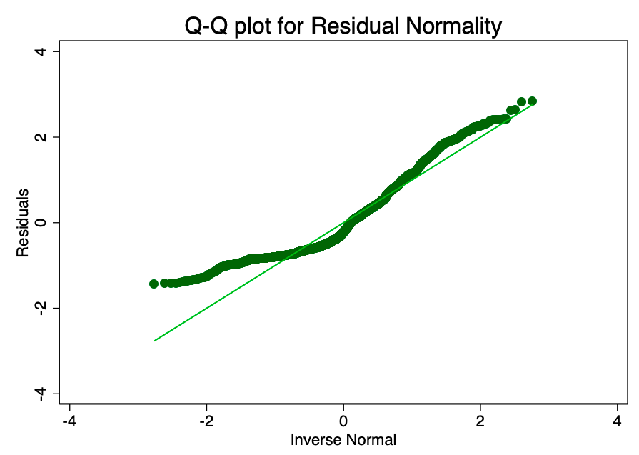
Fig. 9 is a graph with normal quantiles of the error value. The closer the dots to the line, the better the normal fit.

Leverage

Leverage is a concept that not alldata points in regression make an equal contribution to the estimation of coefficients. Some points with high leverage can significantly change the coefficient depending on whether they are present or not. Figure 10 clearly shows that there are too many questionable points (above the average balance and above the average leverage).

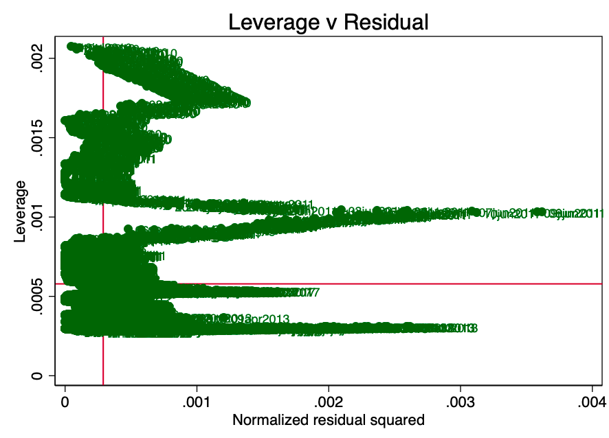
Fig. 10 - Leverage and squared remnants.

OLS Summary

Basic diagnostics indicate a violation of almost all Gauss-Markov conditions, with the exception of linearity. This is a pretty strong proof of the failure of H0.

Stationarity

A process with a total order of 0 is called stationary.(eg I(0)). A non-stationary process is I(1) or more. Calculating an integral in this context is more of a poor man's sum of differences with a time shift. I(1) means that subtracting the first lag from each value in the series results in an I(0) process. It is quite well known that regression on non-stationary time series can lead to the identification of spurious relationships.

Figures 12 and 13 below show that we cannotdisprove the null hypothesis of the extended Dickey-Fuller test (ADF). The null hypothesis of the ADF test is that the data is non-stationary. This means that we cannot say that the data is stationary.

</p>

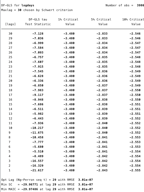
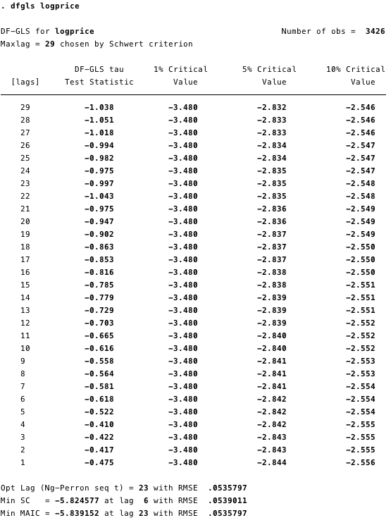
Figures 11 and 12 - Advanced Dickey-Fuller test for a unit root of the logarithm of the price and the logarithm of the number of days.

The Kwiatkowski-Phillips-Schmidt-Shin (KPSS) test is a complementary test for stationarity to the ADF tests. The null hypothesis of KPSS is thatthe data is stationary.As can be seen in Figures 13 and 14, we can refute the stationarity for most lags in both variables.

</p>

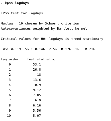
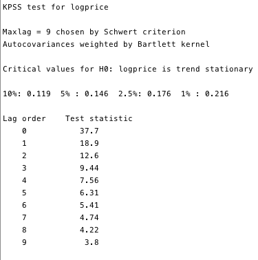
Fig. 13 and 14 - KPSS test against the null hypothesis of stationarity

KPSS tests prove that these two series, outsideall doubt are unsteady. And this, in general, is a problem. If the series is not stationary at least relative to the trend, then the OLS method can identify false dependencies. The only thing we could do was take the difference between the logarithm and the daily value of each variable and rebuild our least squares. However, due to the fact that this question is quite widespread in econometric circles, we have a much more reliable framework called cointegration.

Cointegration

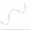
Cointegration is a way to deal with a couple(or more) processes I (1) and determine whether there is a relationship between them and what it consists of. To illustrate cointegration, a simplified example of a drunkard and his dog is often given. Imagine a drunk man heading home, walking a dog on a leash. A drunkard sways in an unpredictable way along the entire width of the road. The dog is also moving rather chaotically: he sniffs the trees, barks, digs something with his paws - such a restless little dog. However, the dog’s range of motion will be limited by the length of the leash held by the drunkard. That is, it can be argued that at any point on the drunkard’s route, the dog will be within the length of the leash from him. (Of course, we cannot predict in which direction from the drunkard she will be at each moment of time, but she will be within the leash.) This is a very simplified metaphor for cointegration - the dog and its owner move together.

Compare this with the correlation: let's say a stray dog ​​follows a drunkard’s dog for 95% of their journey, and then runs away with a bark the other way behind a passing car. The correlation between the routes of a stray dog ​​and a drunkard would be very strong (literally R²: 95%), however, like many random connections of a drunkard, this ratio would mean nothing at all - it cannot be used to predict the location of a drunkard, since for some A fragment of the path, the forecast based on these data will be correct, but for some parts it will be completely inaccurate.

In order to find the location of a drunkard, we first need to understand which lag order specification should be used in our model.

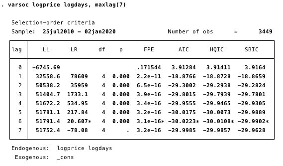
Fig. 15 is a specification of a delay order. The minimum AIC value used to determine.

Here we determine the delay order most suitable for the study by choosing the minimum AIC value of order 6.

Next we need to determine the availabilitycointegrating relationship. With the simple Angle – Granger method (see sources at the end of the original article), this is relatively easy. If the negative statistics of the test exceeds critical values, then there is a cointegrating relation.

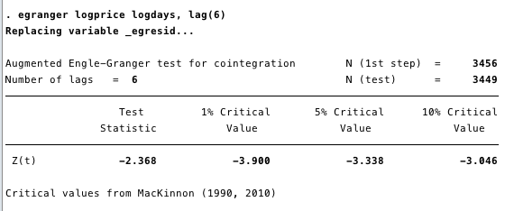
Fig. 16 - Statistics of the test and close to not lower than any of the critical values.

The results in Figure 16 give no reason to state that between the logarithm of the price and the logarithm of the number of days there is a cointegrating equation.

Limitations

In this study, we did not take into account anydistorting factors (confounders). Given the evidence above, it is extremely unlikely that any confounders could have a significant impact on our conclusion - we can reject H0. It can be argued thatthere is no connection between the logarithm of the number of days and the logarithm of the price of bitcoin. If there was such a connection, there would have to be a cointegrating relation.

Conclusion

Violation of all but one of the Gauss–Markov conditions for real linear regression, coupled with the nonstationarity of both variables, provides sufficient evidence forrebuttalsH0, therefore,there is no real linear relationship between the logarithm of price and the logarithm of the number of days, and such a relationship cannot be used to predict price values ​​outside the sample.

 

</p>