Supply and Demand Model for Bitcoin Price

In this article, the author attempts to model the price of Bitcoin as a function of supply and demand. He exploresthe possibility of using a double logarithmic time model for supply and demand and rejects it due to serious heteroscedasticity. Then using the programauto.arima, he finds a fairly productive modelautoregressive integrated moving average. After that, he uses the supply and demand forecast built using ARIMA to model the future price of bitcoin, taking into account the fact that his supply volume is known.

Notes

• Minimum required pre-reading:
  • https://bitnovosti.com/2019/04/03/modelirovanie-tseny-bitkojna-ishodya-iz-ego-defitsitnosti/
  • https://bitnovosti.com/2019/09/27/falsifitsirovanie-koeffitsienta-stock-to-flow-kak-modeli-stoimosti-bitkojna/
  • https://ru.wikipedia.org/wiki/Demand Law
• The analysis was performed using Stata 14 and R 3.4.4
• Not a financial recommendation.
• All models are incorrect, but some of them are useful.

Introduction

The ratio of stocks to growth (Stock to Flow), the designation of which here we will abbreviate for convenience toSt / f, as has been proved (1, 2), is a false predictor of the price of bitcoin.

A common criticism of price modeling usingSt / fThe problem is that it does not take into account the influence of demand. After all, price is a function of supply volume.anddemand. INSt / fsupply is modeled, but how do models built on the basis of this metric react to changes in demand?

In this article, we will take for absolutetruth two ideas, even though they may not be. We will call these truths axioms, and we will formulate these axioms so as to establish some basis on the basis of which it will be possible to develop a model of supply and demand.

Legend

Traditionally, the calculated value of a statistical parameter is indicated by a «cap» above the symbol. Here we will use [ ] instead, i.e. calculated valueβ= [βMatrix 2×2 will be represented as [r1c1, r1c2, r2c1, r2c2], and so on.To denote indexed elements, we will use the @ symbol – for example, for the 10th position in vector X, X is usually used with a subscript of 10.Instead, we'll be writing X@10.

Axiom 1: Price is a function of supply and demand

Quoting the English-language Wiki,

In microeconomics, supply and demand areeconomic model of market pricing. It is postulated that, ceteris paribus, in the competitive market, the unit price of a certain product or other object of trade, such as labor or liquid financial assets, will change until it reaches the point at which demand (for the current price) is equal to supply ( at the current price) and the economic balance will not be established.

Assume that: price (P) = demand (D) / sentence (S). An increase in supply with a constant level of demand leads to a decrease in price. Growing demandDat a constant level of supply leads to an increase in price.

Here we determine the increase in the amount of the asset (flow in the coefficientSt / f) as monthly growth to avoid confusion withlong-term effects. Now let's assume that the supply side of Bitcoin is modeled from the inverse of scarcity (i.e. abundance), i.e.S = 1/St/F +ε = F/St+ε,Whereε– this is some arbitrary error. Our price equation in this case will look like this:P=D/ (F / St + ε). Let us also assume that demandDis also a derivative. And suppose thatεis an independent and randomly distributed value, with an arithmetic mean of about 0.1, and therefore can be (for now) ignored in the model.

Then we get thatP = D/(F/St),from which it follows thatD = PF / St.

Axiom 2: Demand is a function of time t

Let's add a condition that demand is modeled by some function of timef (t) = D = βt.

Regular Least Squares Regression (OLS) -This is a method of finding a linear relationship between two or more variables. To begin, let's define a linear model as some function X, which is equal to Y with some error:

Y = βX + ε

where Y is the dependent variable, X is the independent variable,εis the magnitude of the error, andβ– multiplierX. The job of OLS is to output the valueβso as to minimizeε.

In order to derive a reliable calculated value [β], it is necessary to observe some basic conditions:

1. The presence of a linear relationship between dependent and independent variables
2. Homoskedasticity (i.e. constant dispersion) of errors
3. The average value of the error distribution is usually zero
4. Lack of autocorrelation of errors (that is, they do not correlate with the sequence of errors taken with a time shift)

Now we can calculate[D]using a least squares model[D] = [β] t + ε.

Linearity

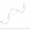
First, take a look at the unaltered scatterplot for the relationship of demand to time.

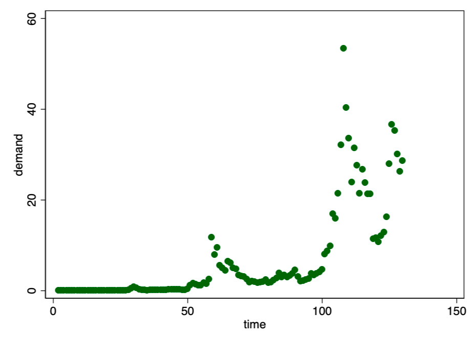
Figure 1. The relation of demand to time looks as potentially exponential.

In Figure 1 we see a familiar pattern of exponential growth. For such cases, as a rule, the double logarithmic model is well suited (Figure 2).

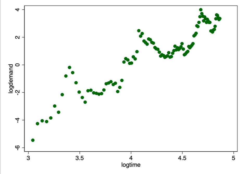
Figure 2. A straight line in a double logarithmic plot indicates a good match for the exponential ratio.

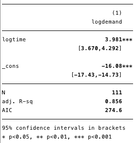
Figure 3. Bootstrap double logarithmic regression (using robust estimation for variance)

As shown in Figure 3, our calculated value islog([D])=3.98log(t) -16,from which we can conclude that for each 10% increase over time, we expect an increase in demand by 46% (eg1.10 ^ 3.98 = 1.46)

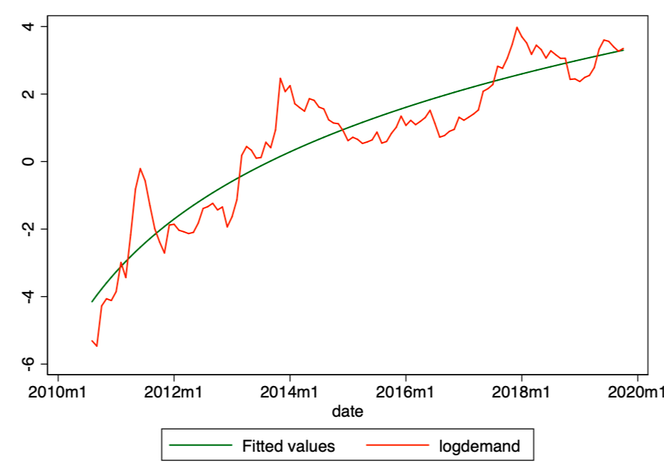
Figure 4. Estimated values ​​(green line) and actual logarithmic demand values ​​(red line).

Using this model, we can now determine the residuals [ε] and calculated values ​​[Y], and also check compliance with other conditions.

Homoskedasticity

If the condition of constant dispersion inthe magnitude of the error (i.e., homoscedasticity), the error for each value of the predicted cost fluctuates randomly around zero. Therefore, the graph of the ratio of residual value to estimated value (Fig. 5) is a simple and effective way to graphically verify the fulfillment of this condition. In Figure 5, we observe a distinct pattern rather than random scattering, indicating significant variability in the variance in the magnitude of the error (i.e., heteroskedasticity).

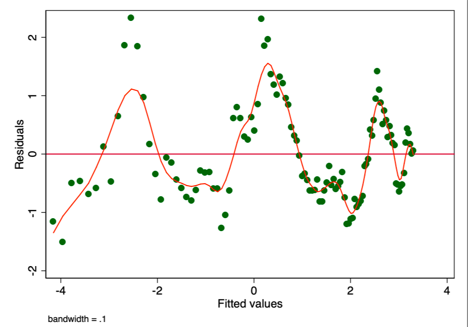
Figure 5. Graph of the ratio of residual value to estimated value. The presence of a pattern indicates a possible problem.

The consequence of such heteroskedasticity is a much larger dispersion and, accordingly, lower accuracy of the calculated values ​​of the coefficients [β]. In addition, it leads to an exaggerated significance of p-values, since the OLS method does not reveal increased variance. Therefore, to calculate t- and F-values, we use an underestimated dispersion value, leading to a higher (unreliable) significance. It also affects the 95% confidence interval for [β], which is also a dispersion function(via standard error). To try to improve this situation, we used the robust sandwich estimator (Huber estimator) to determine the amount of variance and bootstrap (a form of resampling) the regression. However, these results indicate that even after all the adjustments made, we still cannot trust the results of this ordinary least squares test. It can be said that every OLS time-price model (such as the one shown here) is susceptible to this problem. Therefore, instead of it, we will explore another, more suitable time model - the ARIMA model.

ARIMA

More suitable than simple time regressionor its variations, ARIMA is a method designed to model changes in time series over time. ARIMA is an abbreviation for Auto Regressive Integrated Moving Averages, which translates as «autoregressive integrated moving averages». This method includes a whole class of models that explain time series based on their own past values ​​- such as lags or lagged forecast errors. Any time series that exhibits some pattern and is not random white noise can be modeled using an ARIMA model (or a modified version of it).

The basic ARIMA models are defined by three members: p, d, q,

Where:

• p is the autoregressive order (AR),
• q is the order of the moving average (MA) and
• d is the number of differentiations required to make the time series stationary (I)

Using an R programauto.arimafrom the forecast package allows you to selectARIMA model that meets the Akaike Information Criterion - the program tries various combinations of p, q and d and finds the best match. Here we can see that the program has chosen an autoregressive order of 3, a moving average order of 1, and an integration order of 2 (interestingly,auto.arimauses the KPSS test to determine the optimal order of integration, already familiar to those who have read the article about falsifying the coefficientSt / f)

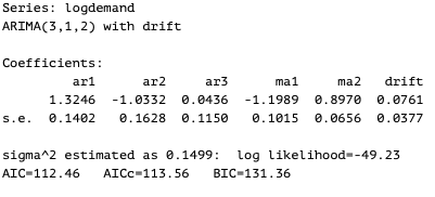
Figure 6. R auto.arima program automatically selected the best parameters for ARIMA.

In Figure 6, we determined the coefficients for ARIMA.

Figure 7. The degree of statistics compliance for the model shown in Figure 6.

Now, watching the square root ofThe standard error of the model (RMSE) in Figure 7, we expect the formation of a small difference between projected and actual demand. The graph in Figure 8 clearly shows that this model estimates historical demand much more accurately than OLS.

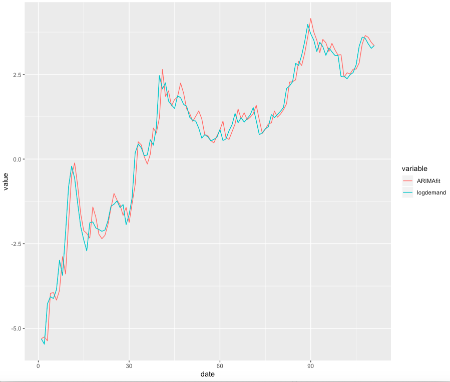
Figure 8. The calculated ARIMA values ​​for the logarithmic demand values. The level of compliance is much higher than when using the OLS method.

The process of creating a dynamic forecast from ARIMAit is difficult to express here in the form of formulas, but if you are interested in studying this question in full detail, then take the time and familiarize yourself with these works: 1, 2 (English).

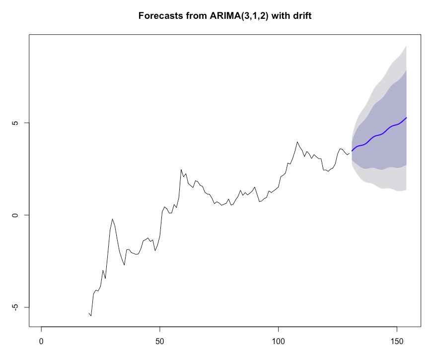
Figure 9. ARIMA forecast for the logarithmic demand values ​​for the next 2 years.

How does our demand forecast look on a linear scale?

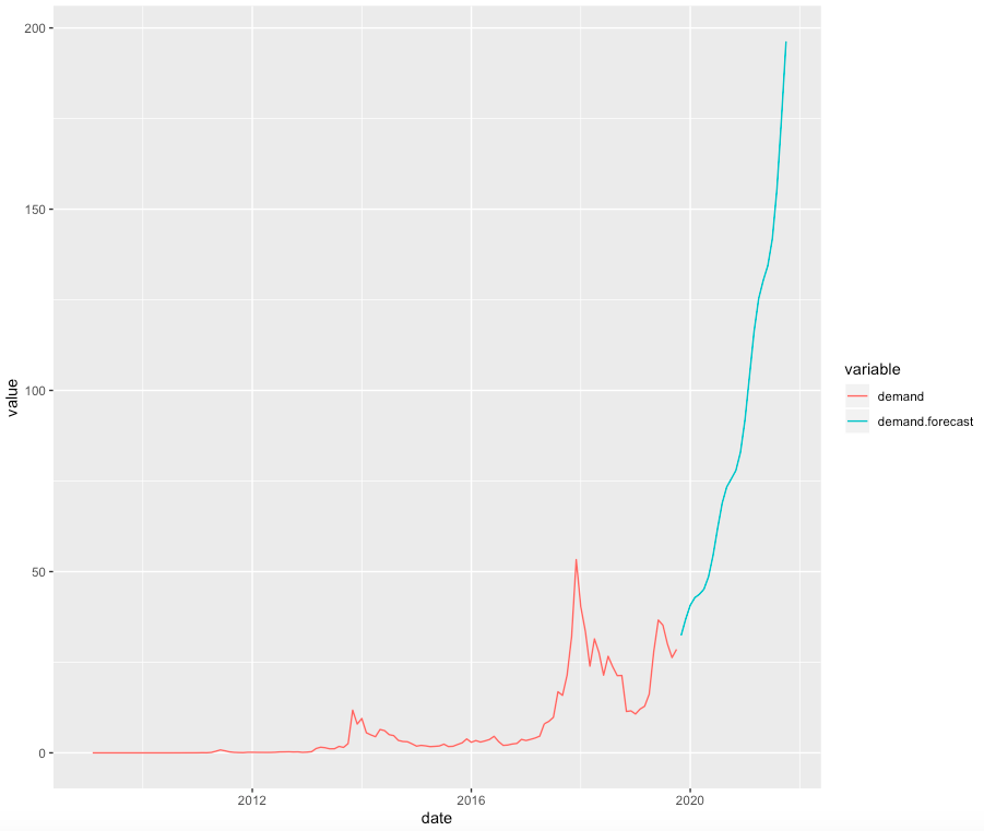
Figure 10 - Forecast of supply and demand from ARIMA in linear space.

Connection models

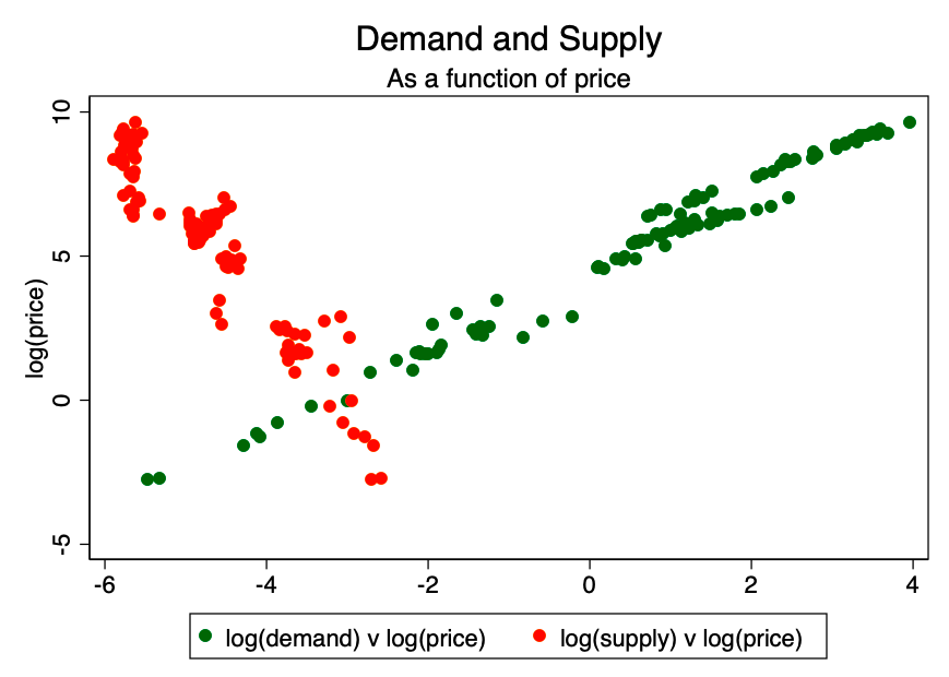
Figure 11. Demand and supply depending on the price.

Now we can combine our forecast data and the expected values ​​of stocks and growth (amount of asset) to calculate the forecast price.

Previously we established thatP = D/(F/St)see axiom 1.

We know what they will be (with a slightmargin of error) growth and stocks over time, so we can combine these numbers with the demand forecast obtained using ARIMA. The result is shown in Figure 12.

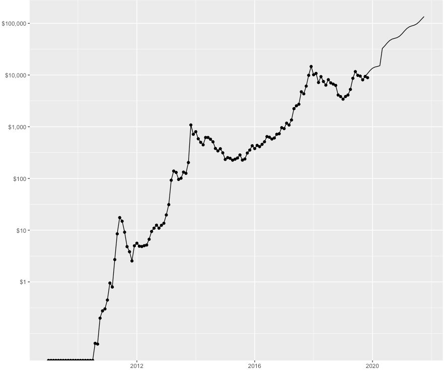
Figure 12. The actual price is marked with dots, the price of the model with a line. As you can see on the chart, according to this model, we can expect that the price of bitcoin will exceed $ 100,000 by the end of 2021.

Conclusion

We presented a simple and relatively concisea supply and demand model for the price of Bitcoin, in which supply is modeled on the basis of abundance (that is, from the opposite to the deficit, determined through the ratio of stocks to growth). This basic model has the potential to expand, in particular by studying demand models based on variables other than time.

Warnings

• This forecast relies heavily onARIMA. ARIMA calculations may turn out to be incorrect - forecast models often turn out to be erroneous. They are nothing more than a way to simplify reality in such a way as to help us better understand it. In this article, we tried to simulate the price of bitcoin as a derivative of supply and demand.
• We did not perform any diagnostic teststo validate ARIMA, and how much confidence to place in the results presented is left entirely at the discretion of the reader. Our goal was only to find a way to model price as a function of supply and demand, not to findthe bestsupply and demand model. This problem is left as an exercise for the inquisitive reader.
• In addition, our second axiom may well be wrong. Time can be a good substitute for a true acceptance curve, but it is unlikely that demand alone could be explained to them.
• The whole idea that price is justfunction of supply and demand (i.e., axiom 1), it is likely that it does not fully describe the real state of things. There may well be feedback loops and other structural relationships (as well as emotionality of consumption, etc.) that are not taken into account in this simple equation. Stay tuned for further development and research into potential structural relationships.

 

</p>