In this article, the author tries to answer the question: is there a relationship between the ratio of stocks togrowth (Stock-to-Flow, or S2F) and costbitcoin. He checks the proposed PlanB double logarithmic model for statistical reliability, based on the least squares method, for the invariance in time of each of its variables and for possible false dependencies. The Vector Error Correction Model (VECM) was created and tested on the basis of the initial model of the ratio of stocks to growth. Although some of these models are superior to the original from the point of view of the Akaike information criterion, they all cannot refute the hypothesis that the ratio of stocks to growth is an important and uncomplicated predictor of the price of bitcoin.
Introduction
The scientific method is difficult for most people.It is counterintuitive and therefore may lead to conclusions that do not reflect the views of the authors. In order to understand this method, it is necessary to understand and accept its fundamental idea:make mistakes normally. This should be taught at school. If we are afraid to make a mistake, we can never offer anything new. The history of scientific discoveries is full of happy coincidences. Random finds and discoveries can be just as (or even more) important than what they were working on at that moment. Ideas may be erroneous or unconvincing, but what is discovered in the process of testing them creates the foundation for followers.
According to the great philosopher of science CharlesPopper, testing a hypothesis to see if it is wrong is the only reliable way to add weight to the argument that it is true [1]. If rigorous repeated tests cannot prove that a hypothesis is wrong, then with each such test the probability that it is true increases. This concept is called the falsifiability (or potential falsifiability) of a theory. In this article, I will attempt to rig the Stock-to-Flow model of Bitcoin price discovery described in the PlanB article «Modeling Bitcoin Price Based on Scarcity» [2].
Problem definition
To falsify a hypothesis, you must first establish what it consists of:
Zero Hypothesis (H0): Bitcoin value is a function of its Stock-to-Flow coefficient
Alternative hypothesis (H1): Bitcoin value is not a function of its Stock-to-Flow coefficient
PlanB in his article [2] decided to check H0,correlating Regular Least Squares Regression (OLS) on the natural logarithm of Bitcoin's market capitalization and the natural logarithm of the Stock-to-Flow coefficient. The author did not present any concomitant diagnostics, nor any specific reason for the logarithmic transformation of both variables, except for the idea that the double logarithmic model can be expressed as a power dependence. Being non-stationary, this model does not take into account the possibility of establishing false dependencies.
Method
In today's article, we will look at this model,we will diagnose normal regression and determine whether the transformation of the logarithm was necessary or appropriate (or both), and also examine possible interfering factors (confounders), interactions, and sensitivity.
Another issue we are exploring isnon-stationary problem. Stationarity (invariance in time) is a prerequisite for most statistical models. This refers to the idea that if a trend relative to time is absent in average values (or variance), then it is absent at any moment in time.
In addition to stationarity analysis, we are also exploring the possibility of cointegration.
Legend
Traditionally, the calculated value of a statistical parameter is indicated by a «cap» above the symbol. Here we will use [ ] instead, i.e. calculated valueβ= [β].We will represent the 4×4 matrix as [r1c1, r1c2 r2c1, r2c2], etc. To denote indexed elements, we'll use the @ symbol—for example, for the 10th position in a vector X, we'd typically use X with the subscript 10. Instead, we'll write X@10.
Ordinary Least Squares (OLS)
Regular least squares regression is a method of finding a linear relationship between two or more variables.
First, let's define a linear model as some function X, which is equal to Y with some error.
Y = βX + ε
where Y is the dependent variable, X is the independent variable,εis the magnitude of the error, andβ– multiplierX. The job of OLS is to output the valueβso as to minimizeε.
In order to derive a reliable calculated value [β], it is necessary to observe some basic conditions:
- The presence of a linear relationship between dependent and independent variables
- Homoskedasticity (i.e. constant variance) of errors
- The average value of the error distribution is usually zero
- Lack of autocorrelation of errors (that is, they do not correlate with the sequence of errors taken with a time shift)
Linearity
Let's start by looking at the non-scatterplotted ratio of market capitalization and S2F ratio (data from source [4]).
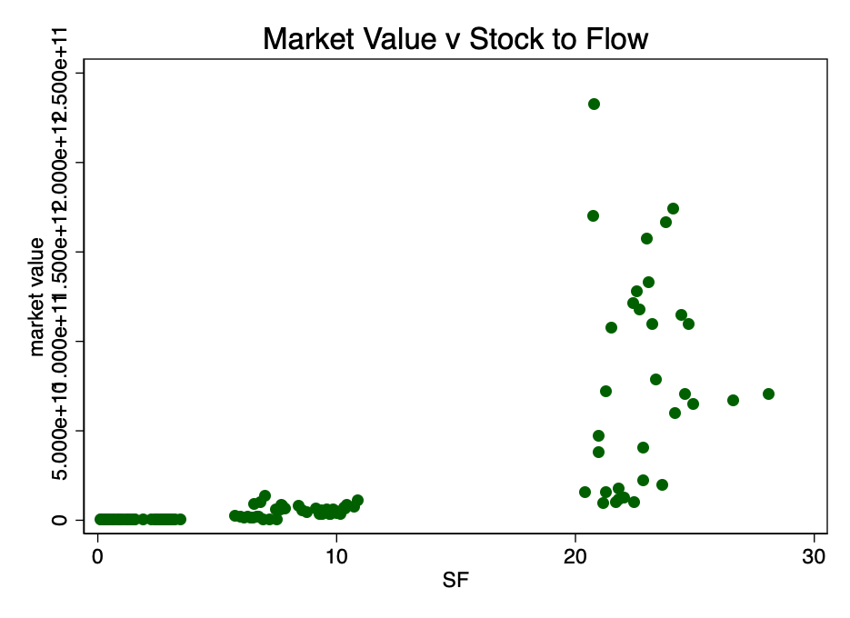
Fig. 1 - The ratio of market capitalization to stock-to-flow ratio. The data is too scarce to be able to establish a relationship.
Figure 1 clearly shows sufficient reason fortaking the logarithm of market value: the range of values is too large. When taking the logarithm of the market value (but not S2F) and re-plotting the chart, we get a familiar pattern (Figure 2).
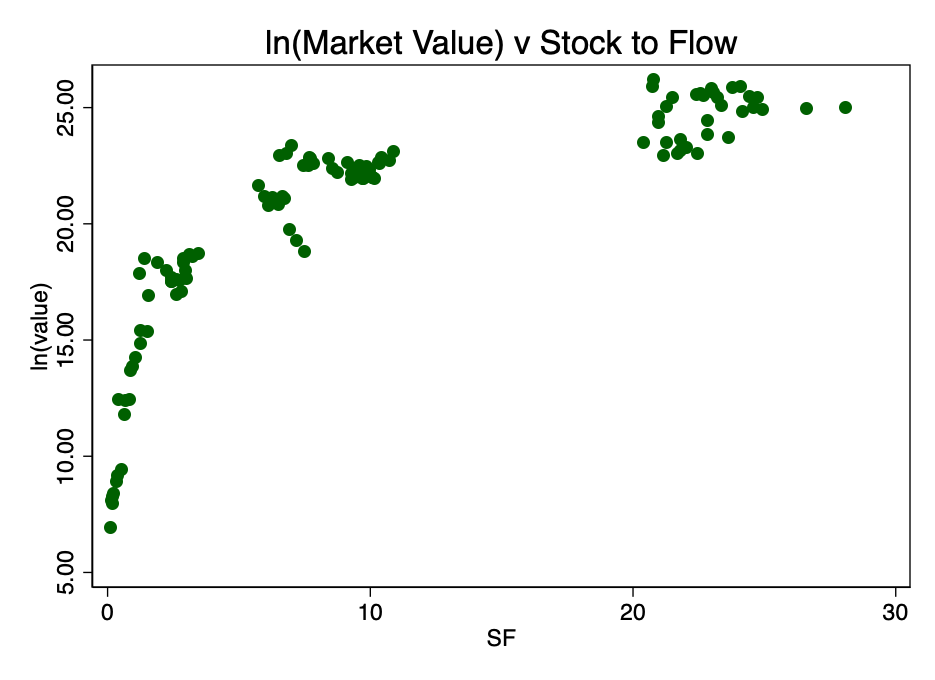
Fig. 2 - the ratio of the logarithm of market capitalization and the coefficient S2F. A distinct logarithmic pattern arises.
Taking the logarithm of the coefficient S2F and constructing a diagram already with it, we get an obvious linear pattern identified by the author of the source [2] (PlanB) in Figure 3.
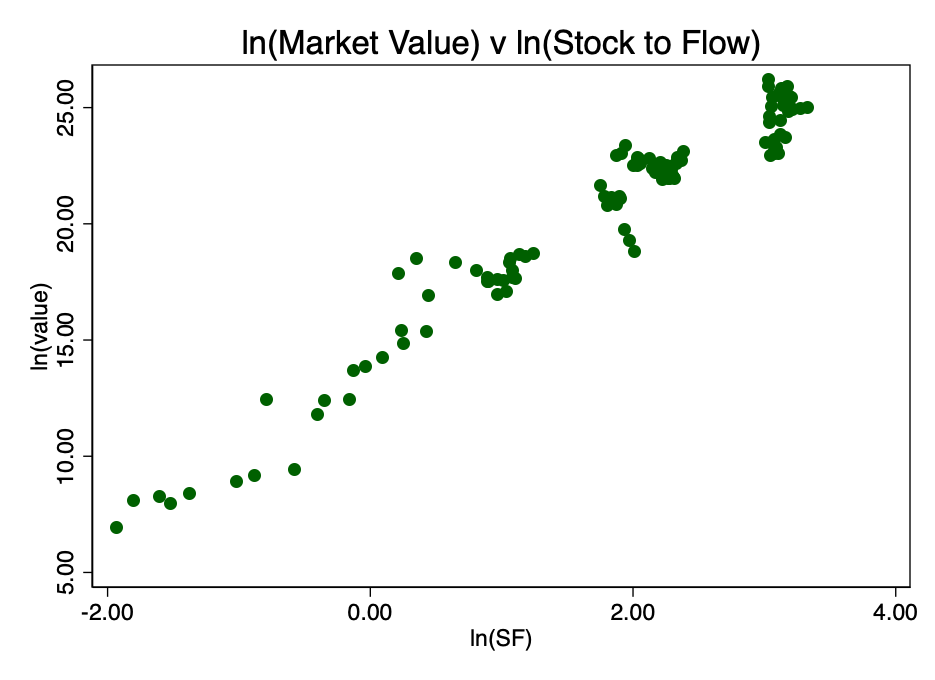
Fig. 3 - the ratio of the logarithms of market capitalization and the coefficient S2F. There is an obvious linear relationship.
This confirms the correct choice of the double logarithm as the only option that results in a well-visible linear relationship.
An alternative transformation was finding the square root of both parameters. The resulting pattern is shown in Figure 4.
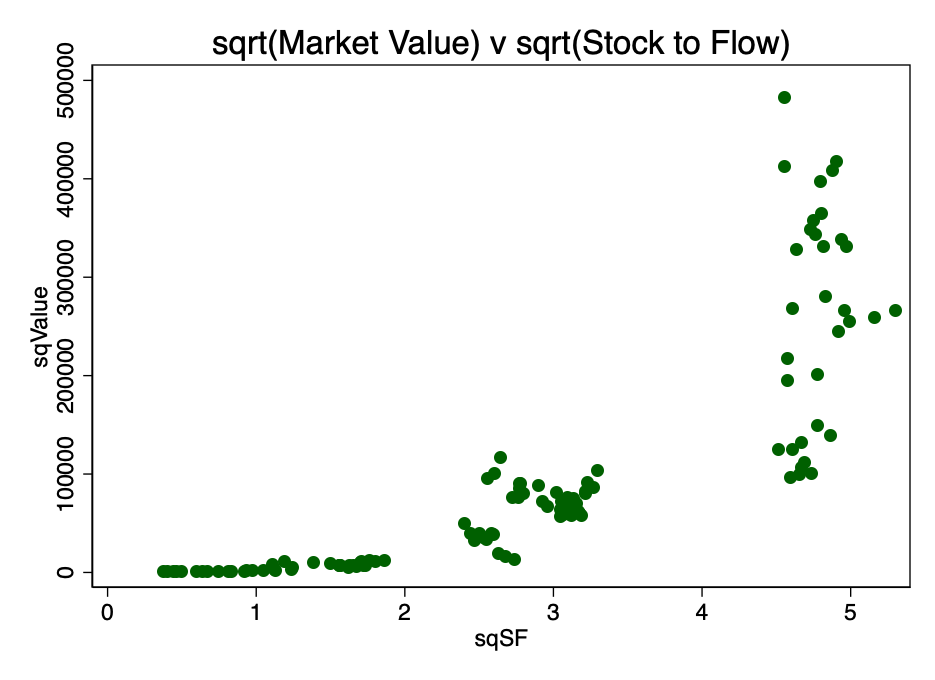
Fig. 4 is a conversion result by calculating the square root of market capitalization and S2F.
Obviously, double logarithm is the most suitable transformation to satisfy the first condition, linearity.
Thus, preliminary analysis does not refute H0.
The results of the double logarithmic regression are shown in Figure 5 below, where [β] =[3.4, 3.7](95% confidence interval).
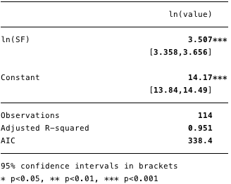
Fig. 5 - results for double logarithmic regression.
Using this model, we can now determine the residuals [ε] and calculated values [Y], and also check compliance with other conditions.
Homoskedasticity
If the condition of constant dispersion inthe magnitude of the error (i.e., homoscedasticity), the error for each value of the predicted cost fluctuates randomly around zero. Therefore, the graph of the ratio of residual value to estimated value (Fig. 6) is a simple but effective way to graphically verify the fulfillment of this condition. There is some pattern rather than random scattering in Figure 6, indicating that the variance in the magnitude of the error is inconsistent (i.e., heteroscedasticity).
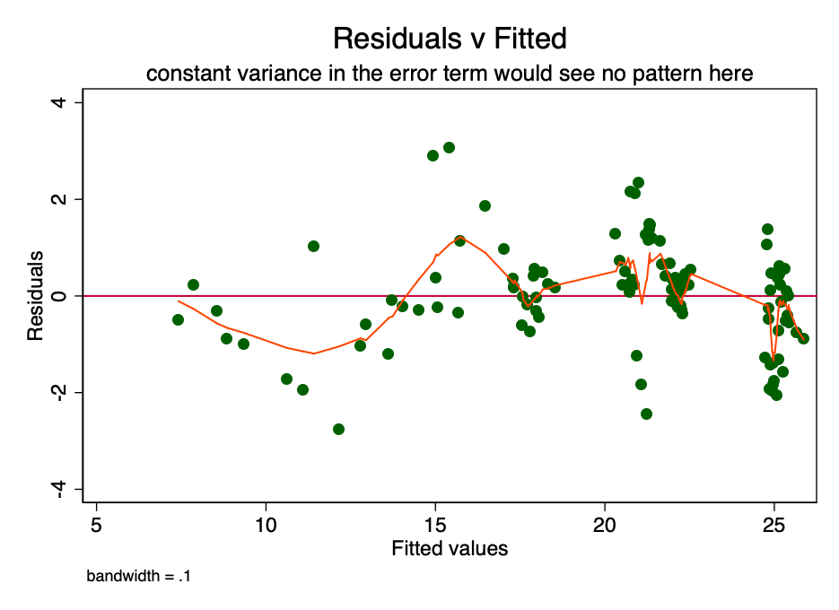
Fig. 6 is a graph of the ratio of residual value to estimated. With a constant variance of the error, the pattern would not be observed. The presence of a pattern indicates a possible problem.
The consequence of such heteroskedasticity is a larger dispersion and, accordingly, a lower accuracy of the calculated values of the coefficients [β]. In addition, it leads to greater than it should be, the significance of p-values, since the OLS method does not reveal increased variance. Therefore, to calculate t- and F-values, we use an underestimated dispersion value, leading to a higher significance. It also affects the 95% confidence interval for [β], which is also a function of variance (through standard error).
You can safely continue at this point.regression, aware of the existence of these problems. There are ways to deal with them - for example, taking bootstrap samples or a robust dispersion estimate.
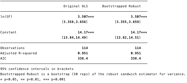
Fig. 7 - The effect of heteroskedasticity is shown in robust evaluation.
As can be seen in Figure 7, despite a smallan increase in variance (see extended confidence interval), by and large, the present heteroskedasticity does not in fact have such a detrimental effect.
At this stage, we cannot refute H0 due to heteroskedasticity.
Normal error distribution
Satisfaction of the condition that the error indistributed with an average value of zero is not as important as satisfying the conditions of linearity or homoskedasticity. With non-normal distribution, but not distorted residuals, confidence intervals will be overly optimistic. If the residuals are distorted, then the final result may be distorted. However, as can be seen from Figures 8 and 9, the residues are within normal limits. The average value seems to be approximately equal to zero, and although a formal test would probably refute the normal distribution hypothesis, the residuals correspond to the normal distribution curve to a sufficient extent so that confidence intervals are not affected.
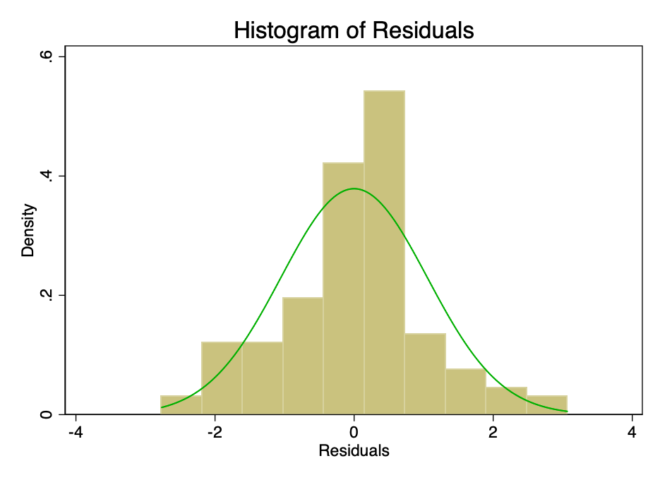
Fig. 8 is a histogram of the error with the (normal) normal distribution curve superimposed on it.
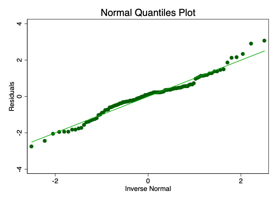
Fig. 9 is a graph with normal quantiles of the error value. The closer the dots to the line, the better the normal fit.
Strength (Leverage)
Leverage here is a concept according to whichnot all data points in a regression make an equal contribution to the estimation of coefficients. Some high impact points can significantly change the coefficient depending on whether they are present or not. In Figure 10 it is clearly seen that in the early stages (March, April and May 2010) there are several questionable points. This is not surprising, and PlanB in his article [2] mentioned that collecting data for an early period was fraught with certain difficulties.
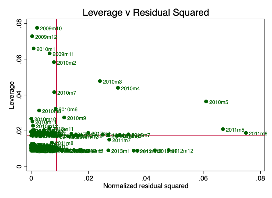
Fig. 10 - impact force and squared normalized residues.
If we restart the regression without these points (suppose there is some kind of error in them), then since we know about the problem of heteroskedasticity, we need to use robust estimates.
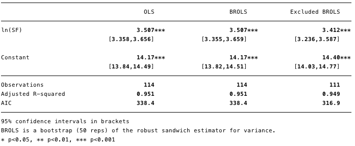
Fig. 11 - the removal of points with a high impact force significantly changed the calculated value [β] and improved the value of the Akaike information criterion (AIC).
Figure 11 shows that the removal of these removal of these three points significantly changes the calculated [β] and the value of the Akaike information criterion is significantly reduced, which suggests that the model is the best, despite the lower R².
OLS Summary
Basic diagnostics point to a few small and fixable problems with the original least squares. At this stage, we cannot refute H0.
Stationarity
A process with a total order of 0 is called stationary.(eg I(0)). A non-stationary process is I(1) or more. Calculating an integral in this context is more of a poor man's sum of differences with a time shift. I(1) means that subtracting the first lag from each value in the series results in an I(0) process. It is quite well known that regression on non-stationary time series can lead to the identification of spurious relationships.
Figures 12 and 13 below show that we cannotdisprove the null hypothesis of the extended Dickey-Fuller test (ADF). The null hypothesis of the ADF test is that the data are non-stationary, that is, it cannot be argued that the data is stationary.
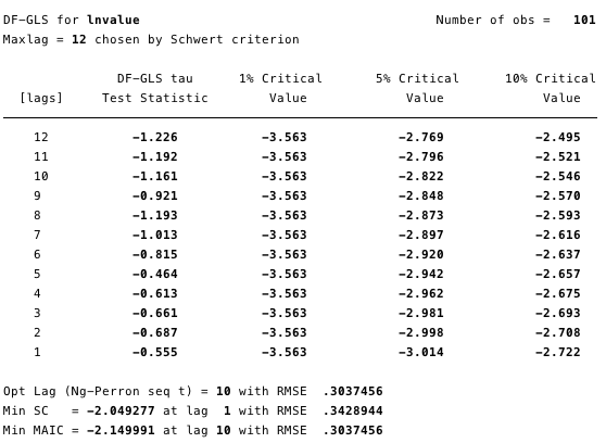
Fig. 12 - extended Dickey-Fuller test for a unit root on ln (cost).
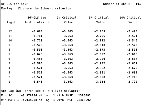
Fig. 13 is an extended Dickey-Fuller test for a unit root on ln (S2F).
The Kwiatkowski-Phillips-Schmidt-Shin (KPSS) test is a complementary test for stationarity to the ADF tests. The null hypothesis of KPSS is thatthe data is stationary.As can be seen in Figures 14 and 15, we can refute the stationarity for most lags in both variables.
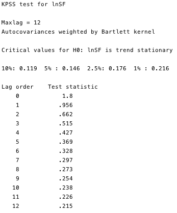
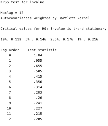
Fig. 14 and 15 - KPSS test against the null hypothesis of stationarity.
KPSS tests prove that these two series, outsideall doubt are unsteady. And there is some problem. If the series is not stationary at least relative to the trend, then the OLS method can identify false dependencies. The only thing we could do was take the difference between the logarithm and the monthly value of each variable and rebuild our least squares. However, due to the fact that this question is quite widespread in econometric circles, we have a much more reliable framework called cointegration.
Cointegration
Cointegration is a way to deal with a couple(or more) processes I (1) and determine whether there is a relationship between them and what it consists of. To illustrate cointegration, a simplified example of a drunkard and his dog is often given [3]. Imagine a drunk man heading home, walking a dog on a leash. A drunkard sways in an unpredictable way along the entire width of the road. The dog is also moving rather chaotically: he sniffs the trees, barks, digs something with his paws - such a restless little dog. However, the dog’s range of motion will be limited by the length of the leash held by the drunkard. That is, it can be argued that at any point on the drunkard’s route, the dog will be within the length of the leash from him. (Of course, we cannot predict in which direction from the drunkard she will be at each moment of time, but she will be within the leash.) This is a very simplified metaphor for cointegration - the dog and its owner move together.
Compare this with the correlation: let's say a stray dog follows a drunkard’s dog for 95% of their journey, and then runs away with a bark the other way behind a passing car. The correlation between the routes of a stray dog and a drunkard would be very strong (literally R²: 95%), however, like many random connections of a drunkard, this ratio would mean nothing at all - it cannot be used to predict the location of a drunkard, since for some A fragment of the path, the forecast based on these data will be correct, but for some parts it will be completely inaccurate.
In order to find the location of a drunkard, we first need to understand which lag order specification should be used in our model.
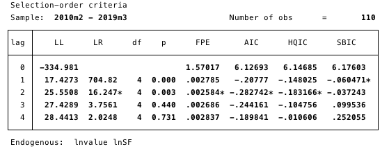
Fig. 16 is a specification of a delay order. The minimum AIC value used to determine.
Here we determine the delay order most suitable for the study by choosing the minimum AIC value of order 2.
Next, we need to determine the presence of a cointegrating relationship. The Johansen framework [5, 6, 7] gives us excellent tools for this.
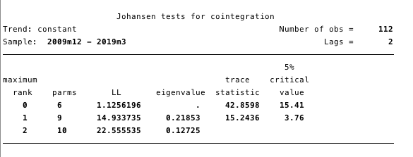
Fig. 17 - Johansen cointegration test.
The results presented in Figure 17 give us reason to assert that there is at least one cointegrating equation between ln (cost) and ln (S2F).
We define our VECM as:
Δy@t =αβ`y@t-1+Σ(Γ@iΔy@t-1)+v+δt+ε@t
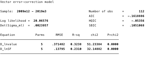
Fig. 18 - information about all equations of the model.
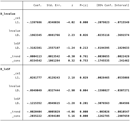
Fig. 19 - calculated values of short-term parameters and their statistics.
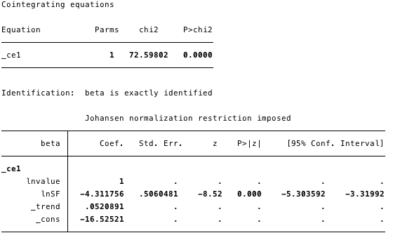
Fig. 20 is a cointegrating equation for the model.
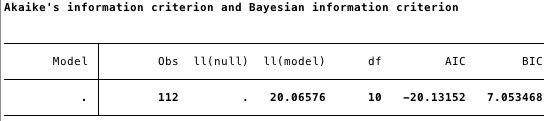
Fig. 21 - Akaike information criterion for VECM.
In the figures above, we have the following calculated values:
- [α] = [-0.14, 0.03]
- [β] = [1, -4.31],
- [v] = [0.03, 0.2] and
- [Γ] = [0.196, -0.095 -0.318, -0.122].
In general, the result indicates that the modelfits well. The coefficient ln (S2F) in the cointegration equation is statistically significant, as well as the correction parameters. The adjustment parameters indicate that if the forecasts from the cointegration equation are positive, then ln (cost) is below its equilibrium value, since the coefficient on ln (cost) in the cointegration equation is negative. The estimated value of the coefficient [D ln (cost)] L. ce1 is -0.14.
So if the value of bitcoin is toosmall, it quickly rises back to the level of correspondence ln (S2F). The estimated coefficient [D ln (S2F)] L. ce1, equal to 0.028, implies that at too low a cost for bitcoin, it is adjusted to an equilibrium level.
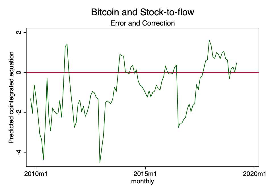
Fig. 22 is a predicted cointegration equation.
The figure above shows that the result of the cointegration equation tends to tend to zero. Although formally it may be unsteady, it definitely tends to be stationary.
From the Stata software user guide:
Accompanying matrix for VECM with K endogenous(intrasystem) variables and r cointegration equations has Kr eigenvalues. If the process is stable, then the modules of the remaining eigenvalues of r are strictly less than one. Since there is no common distribution for eigenvalues, it can be difficult to determine whether they are too close to unity.
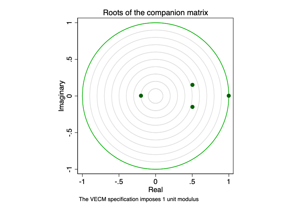
Fig. 23 - roots of the accompanying matrix.
Graphic representation of eigenvaluesshows that none of the remaining eigenvalues is close to the edge of the unit circle. Checking the stability of our model does not indicate its fallacy.
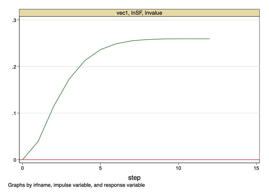
Fig. 24 - impulse response function.
The above figure indicates that the orthogonalized jump to the value of the S2F coefficient has a constant impact on the value of bitcoin.
And at this point we draw the line.The ratio of stocks to growth is not a random variable. This is a function with a known value in time. There will be no jumps in S2F values - its cost can be calculated with accuracy in advance. However, this model provides very convincing evidence that there is a fundamental, unreliable relationship between the value of the S2F coefficient and the value of bitcoin.
Limitations
In this study, we did not take into account anyinterfering factors (confounders). Given the evidence above, it is unlikely that any confounders could have a significant impact on our conclusion—we cannot reject H0. Wecan notassert that there is no relationship between the stock-to-growth ratio and the value of Bitcoin. If this were the case, there would be no cointegration equation.
Conclusion
Although some of the models presented here are withthe points of view of the information criterion, Akaike are superior to the original PlanB model, they all can not refute the hypothesis that the ratio of stocks to growth is an important and uncomplicated predictor of the price of bitcoin.
To illustrate, back to the drunkard metaphorfrom the example above: if we compare the cost of bitcoin with a drunkard, then the Stock-to-Flow coefficient is not the dog that he leads on a leash, but rather the road along which he goes. A drunkard will stagger along the entire width of the road, sometimes he will slip, miss corners or even cut off some corners, but in general he will keep to the road home.
That is, in short, Bitcoin is a drunkard, and the ratio of reserves to growth is the road it goes on.
Quoted Materials
- Karl Popper, «The Logic of Scientific Research» (1959)
- https://bitnovosti.com/2019/04/03/modelirovanie-tseny-bitkojna-ishodya-iz-ego-defitsitnosti/
- Murray, M. (1994). A Drunk and Her Dog: An Illustration of Cointegration and Error Correction.The American Statistician, 48(1), 37–39. doi: 10.2307 / 2685084
- https://github.com/100trillionUSD/bitcoin
- Johansen, S. 1988. Statistical analysis of cointegration vectors. Journal of Economic Dynamics and Control 12: 231–254.
- Johansen, S. 1991. Estimation and hypothesis testing of cointegration vectors in Gaussian vector autoregressive models. Econometrica 59: 1551-1580.
- Johansen, S. 1995. Likelihood-Based Inference in Cointegrated Vector Autoregressive Models. Oxford: Oxford University Press.
- Becketti, S. 2013. Introduction to Time Series Using Stata. College Station, TX: Stata Press.
Notes:
- For all analyzes, Stata 14 software was used.
- The article does not contain financial recommendations.
</p>
Read this:
 Bitcoin hash growth ensured by the launch of 500,000 new ASIC miners
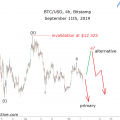 Two weeks ahead of Bitcoin's drop to $ 8,000
 Cryptocurrency mining on ASIC: relevance, profitability, models
 Modeling the price of bitcoin based on its scarcity
 Startup PRISM. Analysis of model development in example No. 1
Bitcoin Social Contract
Startup PRISM. Analysis of model development in example No. 1
Bitcoin Social Contract