Bitcoin's Natural Long-Term Growth Corridor

As the popularity of this cryptocurrency grows, its future value is being increasingly discussed.number of assumptions and conjectures. The forecasts are extremely diverse: some economists, such as Nuriel Roubini, believe that within five years the price of bitcoin will drop to zero, and, for example, John McAfee in his famous prediction predicted $ 1,000,000 for BTC by the end of 2020. Other forecasts fall within this broad range.

In general, the value of bitcoin since its inceptionThe creation in 2009 grew very rapidly, passing through successive cycles of ups and downs. Periods of skyrocketing seem to inspire people like McAfee to make optimistic forecasts about the future price, and long recessions prompt some economists to predict a decline to zero. In this article, we will examine the price dynamics of bitcoin throughout history and make sure that the evolution of its value can be considered as movement within a corridor defined by two power-based dependencies based on time. Although the idea of ​​modeling Bitcoin prices using a power law is not new, here we give an additional justification for it and present several new interpretations.

This model allows us to make several broad forecasts regarding the price of bitcoin in the long term, such as:

• The price will reach $ 100,000 for BTC no earlier than 2021 and no later than 2028. After 2028, the price will not drop below $ 100,000.
• The price will reach $ 1,000,000 for Bitcoin no earlier than 2028 and no later than 2037. After 2037, the price will not drop below $ 1,000,000.

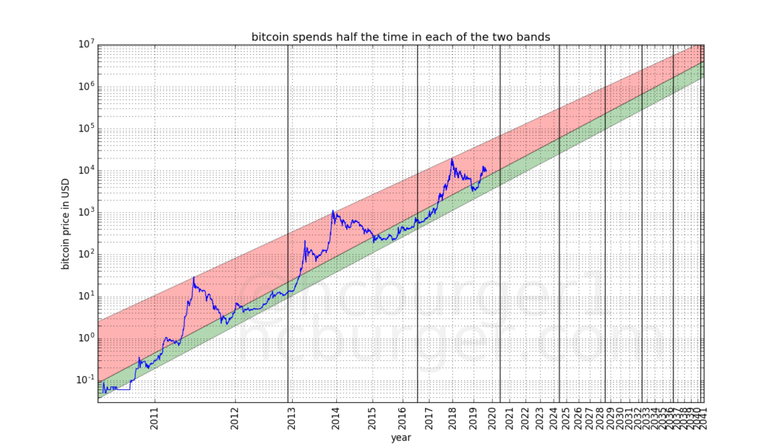
In addition, we will see that the price corridor candivided into two bands, one of which - rather thin - is in the lower part of the forecast price range, and the other is much wider in the upper part. In each of the bands, the price of bitcoin is approximately the same amount of time. And this means that large rallies and recessions, apparently, will continue to occur. The projected ranges may seem quite broad, but they are accurate enough to not coincide with the opposite predictions of some other people. This pricing model also helps identify good entry and exit points.

I am pretty sure that in the long runthe price will really develop approximately as stated in this article. Moreover, I think that these forecasts are more likely to be underestimated than overestimated: I believe that in the case of serious external shocks, bitcoin has a greater potential for growth than for decrease. However, in this article you will not find any forecasts regarding such shock factors. Instead, we will assume that events will continue to develop “as usual”.

Different pricing approaches

The most interesting and amazing aspectThe formation of the price of bitcoin is that over the past few years it has repeatedly grown by several orders of magnitude. The first registered price quote that I could find was $ 0.05 for Bitcoin on the Mt Gox exchange on July 17, 2010, but until that date, a lot of bitcoins were changed hands at a much lower price: for example, May 22, 2010 Laszlo Chanets paid 10,000 BTC for two pizzas, which roughly corresponded to only $ 0.0025 (a quarter of a cent) for bitcoin. At the time of writing this article, the price of BTC is around $ 8,000, which is about 3.2 million times more than the estimated value that Laszlo Haniec once considered acceptable to himself.

Growth by so many orders is quiteunusual for a financial instrument. Indeed, observing a Bitcoin price chart over a large time period can, to some extent, be misleading (if the price chart is presented on a linear scale). Below is a graph of the price of Bitcoin from July 17, 2010 until the beginning of this fall. Similar charts can be found on any site where the price of BTC is given.

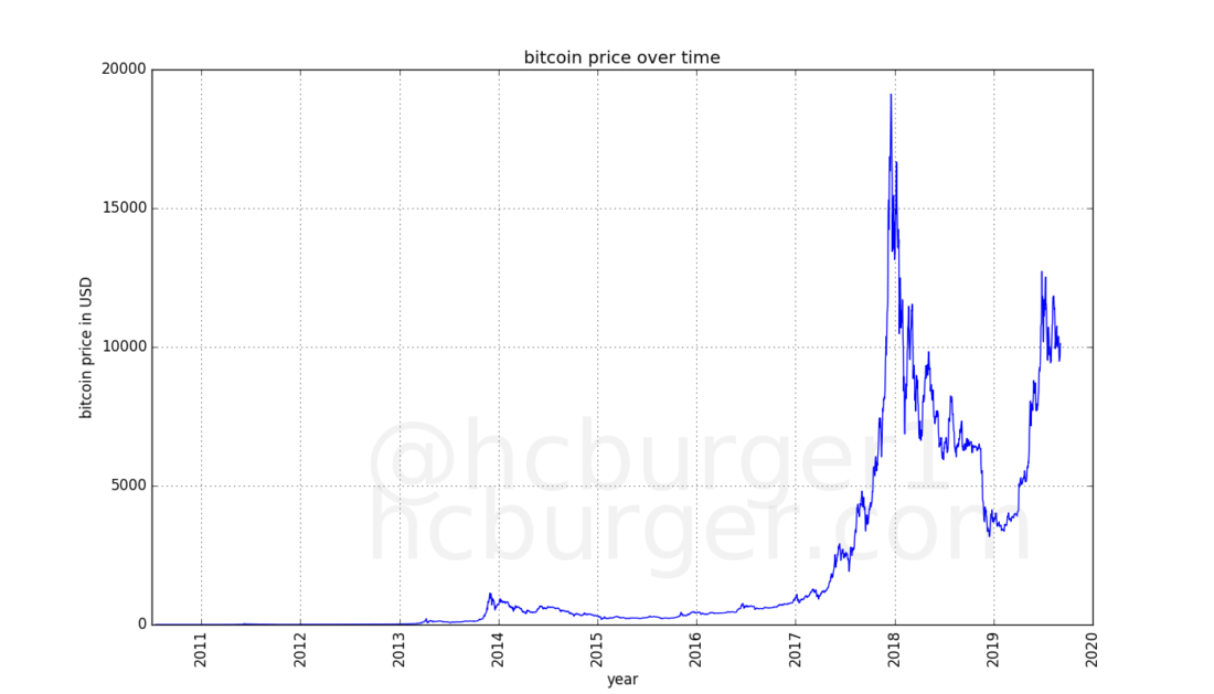
Any price fluctuations closer to todayso great in comparison with prices in the past that they are sometimes barely visible on the chart. However, in order to understand the long-term price trend, it is necessary to take into account all past prices. The linear scale is not suitable for graphically expressing growth by such a number of orders. In this case, it is more advisable to use a logarithmic scale. On a logarithmic scale, the intervals of 0.01–0.1 and 1000–10000 look the same, since they are equal in percentage terms. This allows you to more clearly present the overall picture of the evolution of the price of bitcoin:

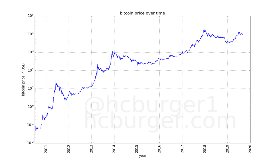
In this graph, it is obvious that the price growth rateBitcoins seem to slow down over time. From $ 0.1 to $ 1 (10 times) the price increased in just a few months. In the future, getting tenfold profit took more time.

In the above graph, the price scale (Y axis) is logarithmic, and the time scale (X axis) is linear. Let's see what happens if the X axis is also made logarithmic:

The price curve takes on an almost flawlessly linear look!

Linear regression

Since this data looks so linearlet's try applying linear regression to them. The idea itself is not new. For example, here's a post on Reddit (English), whose author did exactly the same thing.

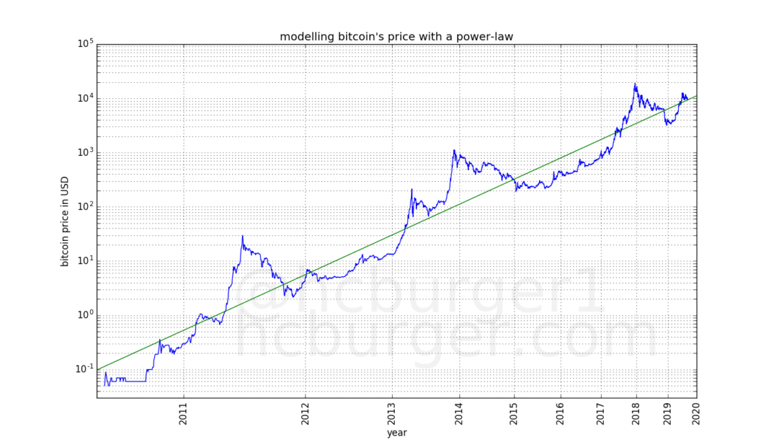
The green line is the result of linear regression. Linear regression allows us to use the following power law to predict the price of bitcoin for a specific day:

where a = -17.01593313, slope b = 5.84509376, and d = number of days since 2009.

Please note: the power dependence is non-linear, since we applied linear regression on logarithmic scales.

Visually, this substitution works«with a bang», and right up to the first prices quoted on the exchanges. Interestingly, the Reddit post was published about a year ago, and the results still look remarkably similar. The coefficient of determination is also high: 0.93139763, which is another confirmation of the correctness of the model selection. We can look at how the coefficient of determination has changed over time. Surprisingly, the model fits the actual data better over time:

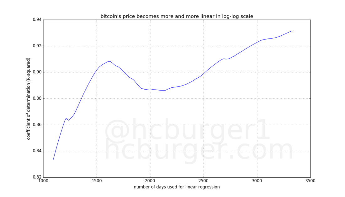
The x-axis represents the number of data points(days) used for the linear regression model, and on the Y axis, an assessment of the model’s compliance with actual data. The price of bitcoin is better and better in line with the power law.

Let's experiment a little more. If we move the above green line a little lower (without changing its slope), we get an excellent support line: Except for the only case in 2010, the price never fell below this line:

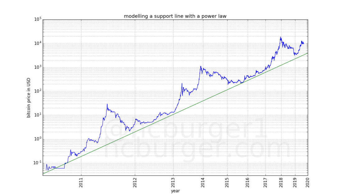
This line looks like a fundamental level of bitcoin price support, which historically followed a power law.

We can also try to build a linearregression only on the three peaks achieved in 2011, 2013 and 2017. It's funny that this lookup also works fine: All three data points are located very close to the line:

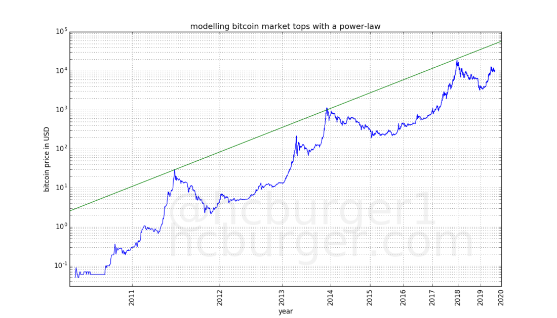
It appears that market peaks also follow a power-law pattern.law. If the next price peak follows the same power law, it will reach this line. The slope of the power law line drawn from the three peaks is 5.02927337, while using all available price data we obtained a slightly larger slope of 5.84509376. This speaks of relative «taming» Bitcoin bull markets compared to the overall trend line. Perhaps this is even expected, because as a mature market develops and the order books become deeper, a decrease in volatility can be expected.

So, we have two power dependencies between which the price of bitcoin moves: the support line and the resistance line, determined by the three peaks of the market.

Now let's see what data pointsbest suited for this model. We'll use random statistical sampling (RANSAC), which is an iterative form of outlier, or noise, removal: First, linear regression is performed on all data points. The data point that least closely matches the specified parameters is then removed and the linear regression is rerun. The process stops when 50% of the data points are removed. The result is shown in this graph:

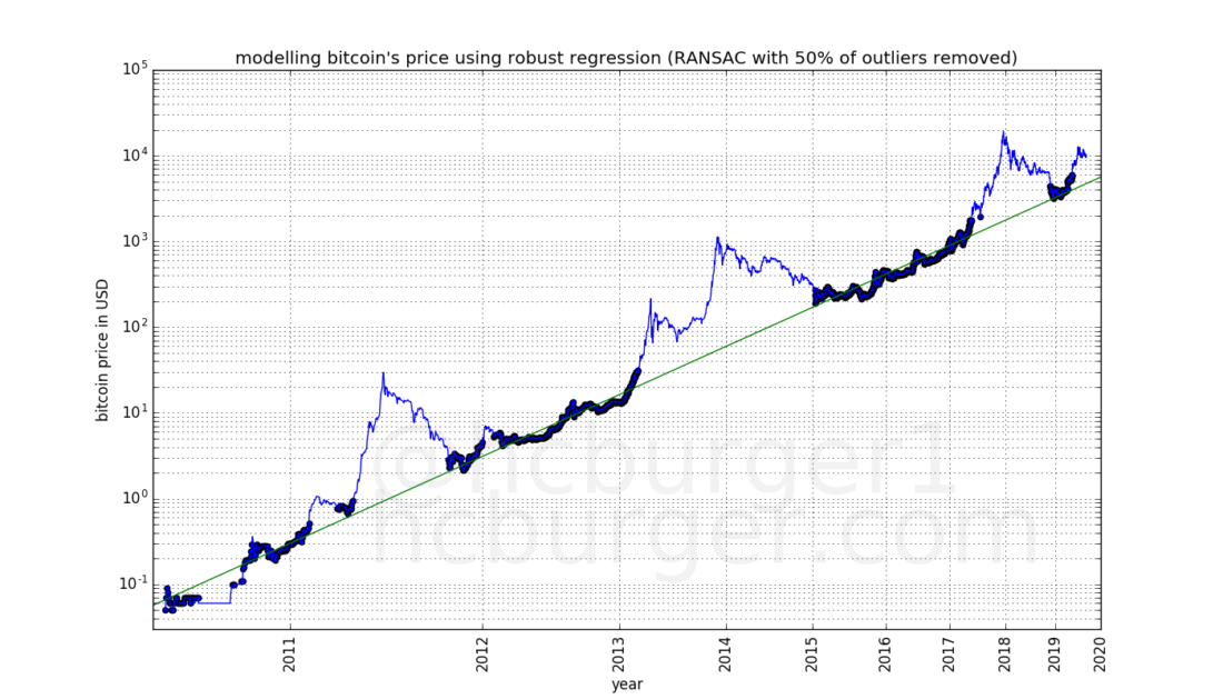
The data points selected by the RANSAC method are highlighted. It seems that the data points are divided into two groups: those that are selected by the RANSAC method are very close to the adapted model; another group includes data points not selected by RANSAC, and almost all of these values ​​are above the adapted model. In fact, some of the points are much higher than the line of the adapted model. Such results arise mainly in bull markets. It seems that Bitcoin price fluctuations have two modes:

• «ordinary», in which the price is very well determined by a power law, and
• «bullish», when the price is more volatile and can rise significantly higher than in normal mode.

In each of the two modes, the price is an equal amount of time.

Finally, we combine all the previously mentioned models in one graph:

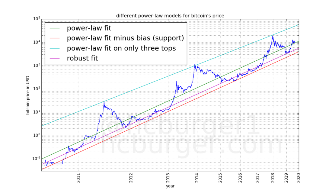
We see that the fitting results are as withUsing all available data, both the RANSAC method have a very similar angle of inclination, but a slightly different offset. This is due to the fact that within the framework of RANSAC, the prices of bull markets were regarded as noise and were almost completely excluded.

Predictions based on developed models

Now we have several models at our disposal to predict the future price of bitcoin. All we need to do is extend the schedule:

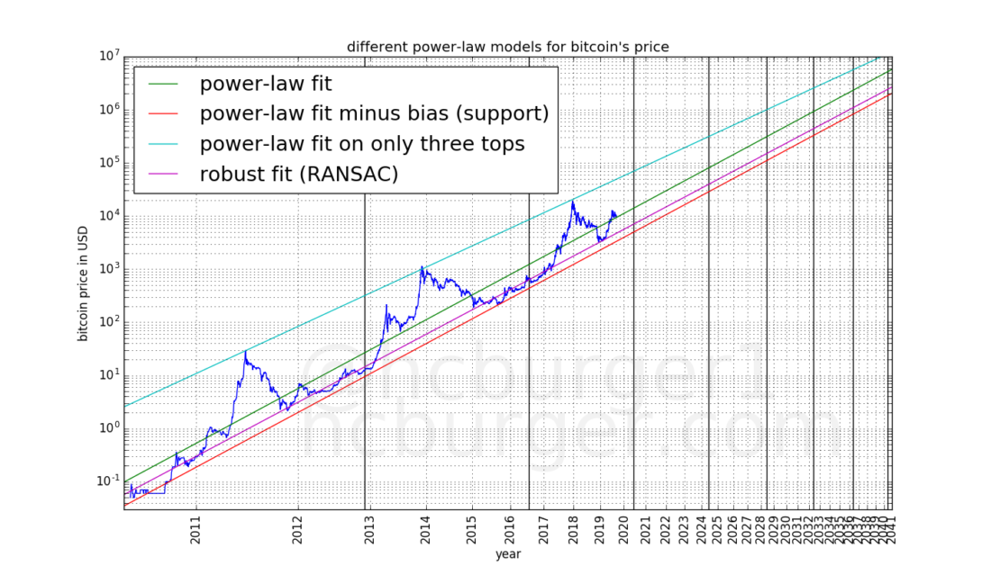
As the model predicts, the price will movebetween the red line of support and the blue line of resistance. The violet RANSAC line defines the middle level of the “normal mode” of the price. Black vertical lines mark two past, as well as expected future halvings.

You can divide the resulting corridor into two bands,one of which corresponds to the “normal” price regime, and the other to the “bullish” one. To this day, the price has been in the lower (green) band of the “normal mode” for half the time, and the rest of the time has been in the upper (red) band of the “bull mode”.

</p>

Interpretation of Results

This power-based modelpredicts that the price of bitcoin will continue to grow in the future, albeit with a slowdown. Volatility, according to the model, will also decrease, although it will remain significant. It is estimated that the price will not reach $ 100,000 until 2021, but it will not be lower than $ 100,000 by 2028. It is estimated that the price will not reach $ 1,000,000 by 2028, but will not fall below this mark after 2037. The model predicts further price increases, although the growth rate will slow down more and more.

These forecasts appear somewhat averaged compared to other forecasts. According to this model, the famous forecast by McAfee is overly optimistic.

The combination of a fairly wide price range anda slowdown suggests that hapless investors will have to wait longer before their initial investment is guaranteed to pay off. For example, investors who purchased bitcoins at the peak of the 2011 boom had to wait about two years before the price finally recovered in 2013. However, investors who bought bitcoins at the peak of the 2013 boom had to wait about four years before the price recovered and fixed at a higher level in 2017. The model predicts that to the level of the highs of 2017, the price of bitcoin is guaranteed to recover in about six years - not earlier than the end of 2023.

So far, in every four-year period of halvinga bubble was forming in the Bitcoin market, the highs of which the price exceeded in the next cycle. But given the slowdown in price growth and the width of the price corridor, a repeat of this scenario is not guaranteed in the future. For example, the model allows the following scenario:

• The price of about $ 150,000 at the beginning of 2022 is part of the next, fourth, four-year period of halving.
• The price is below $ 150,000 until the middle of 2028, that is, until the sixth four-year period.

Such a scenario would provide arguments for criticism to Bitcoin's opponents, but, on the other hand, it can hardly seriously concern those who are ready for such a development of events.

Why the price of bitcoin follows a power law, andis it worth hoping that this will continue in the future? The observation that the price of bitcoin follows a power law, apparently, should be taken as a fact. In addition, there are other factors besides time that should influence the price of bitcoin - such as its scarcity. However, the deficit of Bitcoin is software and, therefore, tied to time. Therefore, it is possible that a simple model based on time will remain relevant in the future. The fact that the power-law fit works better on the logarithmic graph is a sign that this trend may continue.

Conclusion

In this article, we presented simple equations,time-based, to simulate the price of bitcoin. These equations 1) are simple, 2) use time as the only variable, and at the same time work perfectly for a long period of time.

The presented model is not an attemptto predict the onset of bull markets, however, it is expected that price fluctuations on them will be within the price range defined by this model.

Denial of responsibility:The article does not contain financial advice.

</p>