A Non-Divergent Long-Term Predictive Model for Bitcoin Capitalization Based on Residualoffers.
I present to your attention a two-parametera convergent long-term predictive model for Bitcoin that is an alternative to the popular, but mathematically divergent, two-parameter Stock-to-Flow model based on scarcity. Over a 50-year time frame, the price predictions for Bitcoin made by these models differ by 12 orders of magnitude. The Future Supply model is a linear correlation of the logarithm of capitalization with the unissued balance of the total Bitcoin supply (future supply) in any of its "eras".
The mathematical form of this model is inherentlyconvergent, while Stock-to-Flow is the embodiment of a power law of exponential change (since Stock-to-flow changes exponentially with block height), and therefore, by definition, divergent.
R-squared models of future offer onhistorical data amounted to R² = 0.92 for quarterly intervals of 13 125 blocks (1/4 block year). Residues behave well, but have a positive asymmetry. The standard deviation for residuals is 0.374 in terms of the decimal logarithm, reflecting the high volatility of bitcoin.
With the best fit modelconverges to the asymptotic value of capitalization of 1.63 trillion dollars (in 2020 dollars) and the asymptotic price of $ 77,500. However, these values have high uncertainty due to the limited price history and high bitcoin volatility.
By the mid 2020s it will be easy to determine which model is more accurate - the Future Supply model or the ratio of the available supply to its growth (Stock-to-Flow).
PlanB's Stock-to-Flow model is very popular
Scarcity and security are the main drivers of Bitcoin value.
PlanB's Stock-to-Flow (S2F) is the mostA popular prognostic model based on scarcity for bitcoin. She calculates the future price as a function of the S2F coefficient, raising the latter to the third power. The S2F coefficient is steadily increasing with each block, because 1) the amount of available offer relative to the current block reward is growing, and in particular 2) because every 210,000 blocks the block reward for Bitcoin miners is halved. These halving block rewards (halvings) occur at intervals of approximately four years.
The advantage of the S2F coefficient is thatIt is a leading indicator and provides a relatively long-term perspective. It has a fundamental justification in the form of an impact on the asset value of increasing scarcity and has a successful analogue in the precious metals market (the Stock-to-Flow coefficient for gold is approximately 60, and for bitcoin after halving in May 2020, this value will be approximately the same level). The S2F model shows a good correlation with historical data and has withstood several attempts to refute the relationship between the Stock-to-Flow coefficient and the bitcoin price.
The main disadvantage of the model is inherentaccording to the definition of divergence, because the price in it is calculated as a (high) degree of the S2F coefficient, and it steadily tends to infinity (~ 2³⁶ at the last halving, after which - infinity). By 2024, the model will already reach unknown levels, since the S2F coefficient value will exceed 100. For later block eras, the market capitalization predicted under the S2F model increases by 8 times with each halving.
Deficit Modeling Using a Convergent Formula Based on Residual Supply
In this article I bring to your attentionan scarcity-based alternative model that is a function of only the remaining supply. It is designed to be convergent in the long run, with a negative correlation between the remaining issue volume (coins not yet issued) and Bitcoin's capitalization.
For calculations, we used quarterly data starting from block 105,000, that is, after the first two block years. Price data for an earlier period is rather scarce.
The block year represents 52,000 blocks and inan average of about two weeks shorter than the calendar year. The block quarter is 13 125 blocks. Almost 12 block years have passed by today, and the next halving in mid-May of this year will mark the end of the 12 block year, as well as the end of the third and the beginning of the fourth block era.
We examined both power andexponential relationship between market capitalization and future supply. The power-law model, or log (capitalization) / log (future offer), is divergent, since the denominator value tends to infinity (because the remaining emission volume tends to zero). Although such a model has a reasonable R² on historical data, for the moment when the remainder of Bitcoin's supply is reduced to one million coins, it predicts a capitalization of $ 299 trillion. This corresponds to the value of all world wealth, which means that the forecast is untenable.
At the same time, the exponential dependence of the logarithm on capitalization proportional to the future supply of coins is convergent, and our approximation has an anti-correlation of -0.96 and R² equal to 0.92.
We used attitudelog10 (MC) = b + a * f, Wherefis the size of the future supply in millions of coins. Here are the best fit parameters for linear regressionlog10 (MC)Tofon quarter data set: intersectionb = 12,212Anda = -0.3488for the slope (slope). Parameterbis an asymptotic value for log10 (capitalization) sinceftends to zero, and corresponds to a market capitalization of $1.628 trillion. Slope factorbutis the rate of convergence to this value.
This relation can also be written asMC = B * 10 ^ (a * f), WhereB = 10 ^ b, or asMC = B * exp (c * f), Wherec = 2,303 * a. Therefore, for the best fit parameters,MC = 1,628 trillion * exp (-0,803 * f).
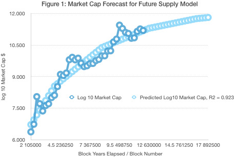
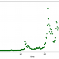
Figure 1: Capitalization Forecast in the Future Supply Model
Observed slope parameter valueaindicates that for every million Bitcoin future supply decreases (and the available supply increases by a million Bitcoins), capitalization increases by10 ^ (0.349) = exp (0.803) = 2.23times.
In Figure 1 above, the blue color indicatescapitalization forecast until the 17th block year (2027 from R. Kh.), and in dark blue - the observed quarterly capitalization from the 2nd block year to the present. Projected capitalization is approaching $ 1 trillion in 2027.
And this is where fundamental «physics» comes into play. – second derivative –as the reduction in future supply is slower over time, the growth of market capitalization is slowing. In the second block era, the future issuedeclined by more than a million bitcoins per year. Now, to reduce future supply by a million coins, it would take about 8 years, or two Bitcoin eras. By 2031, it will take more than a hundred years to reduce future emissions by only 1/3 million bitcoins. In this model, the growth of market capitalization in percentage terms takes more and more time.
In other words, when after the 2024 halvingthe inflation rate will fall below 1% (S2F > 100), market capitalization will no longer be so sensitive to the gradual decrease in the inflation rate. The market will not be interested in Bitcoin's current inflation rate of 0.4%, 0.2% or 0.1%. The difference to dollar supply inflation is what should matter, and the difference between 0.1% and 0.2% would be very small compared to M2 dollar money supply inflation of 5% or 6%. And this also means that we should perceive this forecast in current 2020 dollar values.
The asymptotic capitalization for the future supply model of approximately $ 1.6 trillion is about one fifth of gold capitalization.
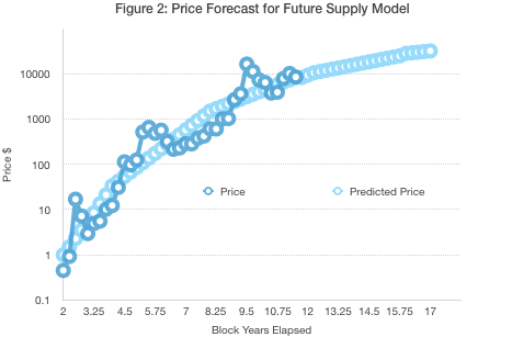
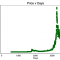
Figure 2: Price Forecast under the Future Offer Model
Capitalization forecast converted to priceforecast by dividing by an affordable offer of bitcoins at each point in the graph in Figure 2. The asymptotic price for this capitalization model is $ 77,538.
Histogram of residuals for actualThe capitalization minus the modeled one is shown in Figure 3. The balances are distributed evenly, with 19 positive and 20 negative values. The standard deviation is 0.374 in the log10 region, which corresponds to a coefficient of 2.37 in both directions. The number of points in the sample of 39 that exceed one standard deviation is 14, against the expected ~ 12.5. The distribution has a positive asymmetry with excessive peak values of the observed capitalization, which is quite expected for several of the strongest bull rallies in Bitcoin history.
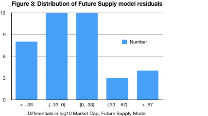
Figure 3: Balance Distribution in the Future Offer Model
However, Bitcoin has a fairly modest price point.history for extrapolating it - we have only 39 points of quarterly data. If you look at the subsets of data, you will find significant variability in the selected parameters a and b. If we exclude the first third of the data points, then the asymptotic price forecast will drop to $ 48,321, and R² will be only 0.69. In particular, the second block era, from 4 to 8 block years, has a smaller slope and a much lower predicted asymptotic price - only $ 8766 - only for this part of the data, while the third (not yet completed) block era gives an asymptotic forecast the price is $ 416,056.
As is usually the case with models, more data is needed here, and only time will tell how useful the model will remain in the future.
Comparison of future offer models and S2F
Let's make a comparison between mathematicallyconvergentmodel of the future supply and mathematicallydivergentStock-to-Flow model.
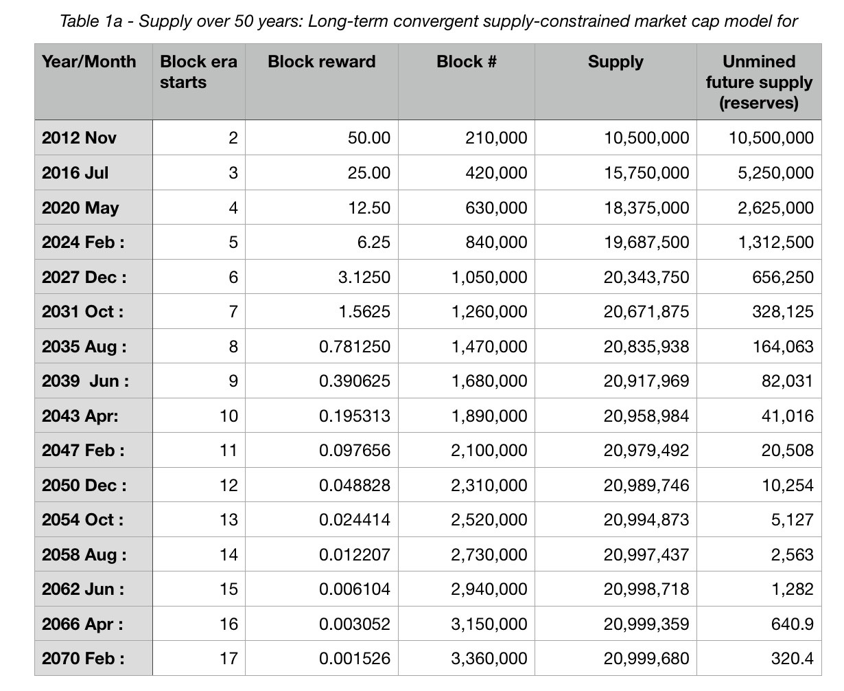
Table 1a - 50-Year Offer: Bitcoin's Long-Term Converged Offer-Based Capitalization Model
Table 1 (a, b) shows the forecast forlong-term convergent model of the future supply. In table 1a above, we give the beginning of each block era over the next fifty years, the size of the block reward, the current offer for each block era, and the remaining issue volume (future offer) for Bitcoin. This is somewhat similar to the existing gold reserves. The difference is that new gold reserves are constantly being discovered or developed, while the volume of future Bitcoin emissions is completely predetermined.
In table 1b, we present the forecast of capitalization andBitcoin prices obtained using the model of the future supply (price = capitalization / stocks or available supply). Notice how projected values grow rapidly in the first few halvings, reaching nearly a trillion dollars by the end of 2027 or the beginning of 2028. But after that, it takes three more halving to reach $ 1.5 trillion, and then the model is smoothed to an asymptotic value of $ 1.628 trillion.
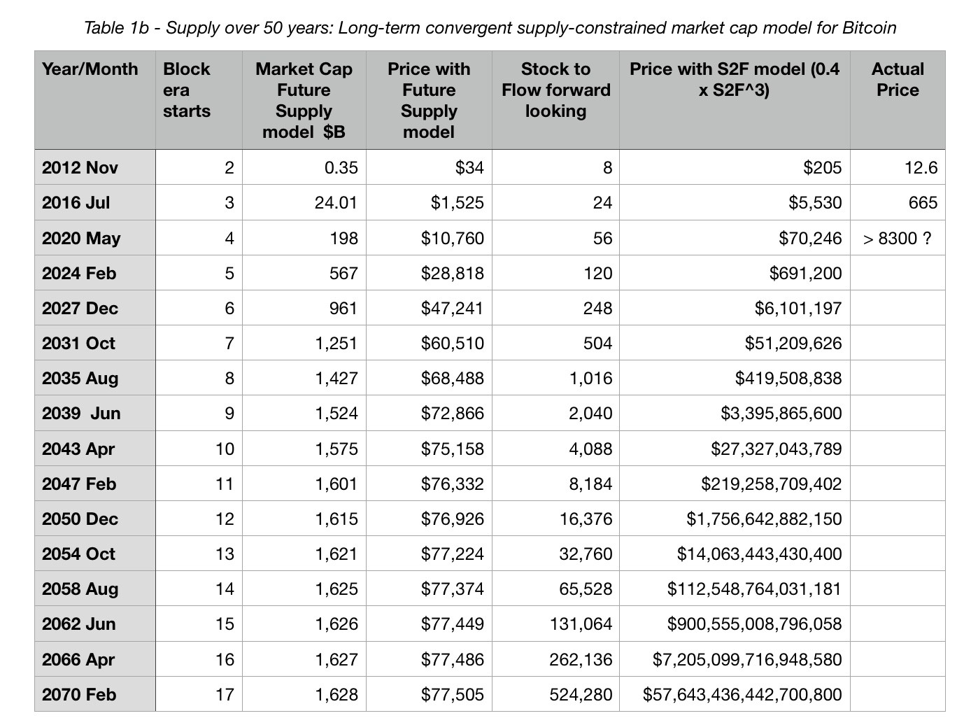
Table 1b - 50-Year Offer: Bitcoin's Long-Term Convergence-Based Offer Capitalization Model
Long-Range Forecastfor the model of the future proposal, approximately corresponds to the forecast of the S2F model for the early 2020s, but never exceeds $ 100,000 for regression on a complete data set. However, since the price volatility coefficient is more than two (one standard deviation), this conditional boundary of $ 100,000 may well be overcome from time to time.
Table 1b also shows the Stock-to-Flow value for each era. The predicted value S2F is given by the identity 4 * (2 ^ E-2), where E is the block epoch indicated in the second column.
And we also give the price predicted at0.4 * S2F³ formula from the original PlanB article (translated here) about the S2F model from March 2019. He also published another version of the model based on annual data and with a power index of 3.3; this version of the model predicts even sharper growth. Capitalization is an almost straight line on the semi-logarithmic price chart for the block era; for a later period, the projected price and capitalization with each new block era increase by 8 times.
We see that the S2F model is becomingunrealistic already in the current decade, since the forecast price before the end of the decade exceeds $ 10 million, which means that the market capitalization exceeds $ 200 trillion, or the value of all real estate on the planet.
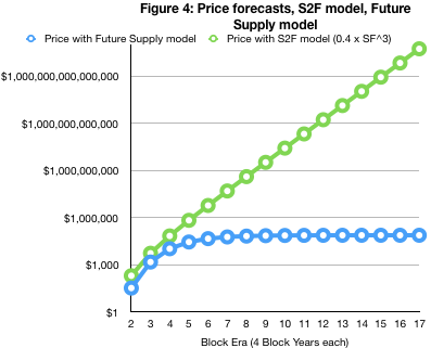
Figure 4: price forecasts obtained in the framework of S2F models and future offers
Figure 4 shows the price forecast for the next 50years (until block era 17, which will occur in 2070), obtained using S2F models and future supply. By the onset of block era 17, model predictions diverge12 orders of magnitude. S2F-predicted priceexceeds 1 billion dollars by the beginning of the 9th block era and 1 trillion dollars by the beginning of the 12th block era. In practice, by the mid-2020s. it will be easy to determine which of the two models is closer to reality.
Model limitations
As I wrote above, there is significant uncertainty in the parameters suitable for the model of the future proposal.
The future offer model does not takeUS dollar supply inflation. If consumer price inflation is around 2%, then the M2 monetary base is growing at about 5–6% per year. So the forecast of market capitalization should be taken as denominated in 2020 dollars. For example, if the M2 monetary base grows by 5% over the next 15 years, the dollar money supply will double, and the forecast for 2035 will be 3 trillion in 2035 dollars.
The model also explicitly ignores the optiona breakthrough adoption, although it indirectly reflects the historically growing number of Bitcoin users and hodlers. If central banks begin to add Bitcoin to their reserves, or if gold yields to Bitcoin the status of a default value preserver, then Bitcoin's capitalization may come close to something comparable to the total value of gold ($ 8 trillion) or even a fraction of the world's foreign exchange reserves ($ 20 trillion).
Bitcoin capitalization idea comparable tocost of total world wealth ($ 300 trillion), it seems to me completely unreasonable, given both the results of the convergent model and the fact that money is not required to express all world wealth. The money supply should support the turnover of GDP, and indeed, the global money supply (like M2) and global GDP are approximately comparable and amount to about $ 90 trillion. Reserve money is a small part of the total money supply.
Conclusion
PlanB's now-successful Stock-to-Flow model predicts that one bitcoin will cost more than $ 1 trillion by 2050 and more than $ 1 trillion by 2070.
Obviously, for a long-term forecast, weI need a more realistic model, and therefore I offer you a model of the future proposal. Its advantages are that it is also based on scarcity, on historical data it behaves comparable to the Stock-to-Flow model, and at the same time it remains convergent even towards the end of this century. In addition, it is very simple, taking only two parameters, has a marginal market capitalization and maintains convergence while reducing emissions.
Such a slowdown in price growth and a decreasevolatility, as it were, is fully consistent with Satoshi's vision of stable global money, which can act as a decentralized reserve for a future scalable payment system. Second-tier solutions and sidechains will increase the scalability of the main blockchain.
A better version of the model of the futureproposals should take into account inflation of the money supply of the dollar, and possibly allow parameterization of the pace of adoption of Bitcoin. But by adoption, I do not mean frequent use for small settlements (high turnover rather reduces cost), but people’s willingness to keep their reserves and savings in Bitcoin, using it as a means of preserving value.
My apologies to those in the next decade.hopes to see BTC for a million dollars, but also in the new model, the predicted return before the beginning of the 8th block era in the mid-2030s still seems extremely favorable. So keep putting off Satoshi. Table 2 below shows the expected return in percentage terms for block eras and block years.
It is still the hardest money ever created.Bitcoin is a store of value, an alternative to money, so itand shouldstrive for stability.If the dollar remains a global reserve currency (perhaps one of several), then the dollar value of Bitcoin should reflect relative inflation rates and relative interest rates (since Bitcoin also develops a credit economy).
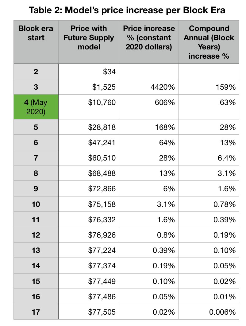
Table 2 - increase the price of the model for the block era
By the mid-2020s, I think we will clearly see which model turns out to be closer to reality - this or Stock-to-Flow.
Appendix: quarterly data
These are the tables with the data underlying the model.future offer. The last column in tables 3a and 3b below shows the difference between observed and simulated capitalization. (Log10 predicted capitalization = log10 observed capitalization minus differential.)
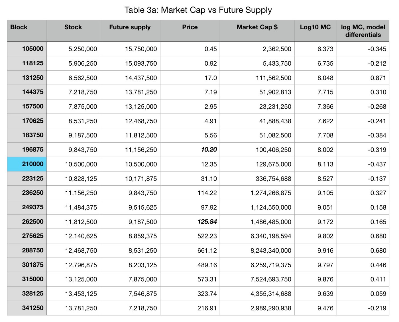
Table 3a - market capitalization and future supply
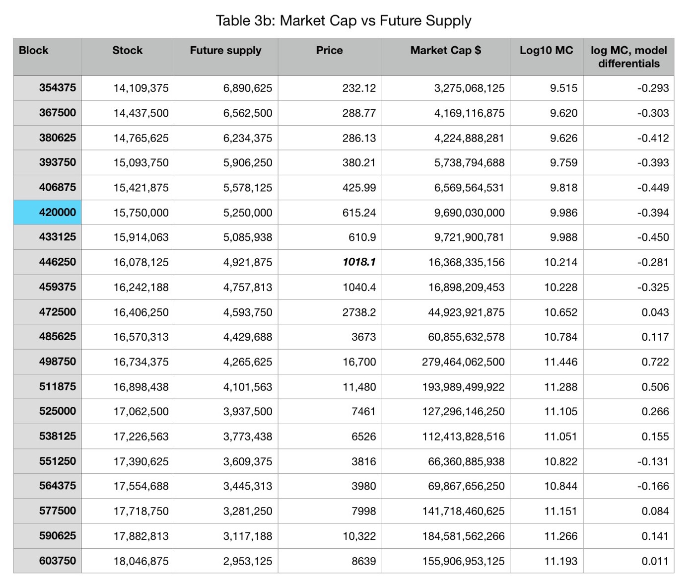
Table 3b - market capitalization and future supply
</p>
Read this:
 Statistical model of stock-to-flow speaks of the beginning of the growth of bitcoin
 Bobby Lee: In a few years, Bitcoin will surpass gold in terms of market capitalization.
 Supply and Demand Model for Bitcoin Price
 Forecast: By 2022, Bitcoin will reach $ 100,000
 Copy-paste | Bitcoin exchange rate falls short of Stock-To-Flow model
 Faking a Logarithmic Bitcoin Price Growth Model