Every week the prison sends me several Bitcoin charts so that I can analyze them and stayup to date (I talked about the context of thisin the first post). These charts go a few days before me and a few days back, so everything published by me may look somewhat irrelevant. However, this is not a problem, because I will analyze only large market movements on a scale of months, years and even decades. In most cases, such an analysis should remain relevant no matter what happened during the sending of the charts, but I will keep this restriction in mind and try to mention, just in case, possible scenarios that may be implemented during this time.
We will consider the graphs of the Bitcoin todollar (see Fig. 1), because the largest trading volume throughout the history of Bitcoin was precisely in dollar pairs. The analysis method I chose, the Elliott Wave, is based on the psychology of the masses (I talked about this in a previous post), so the larger the market, the better.
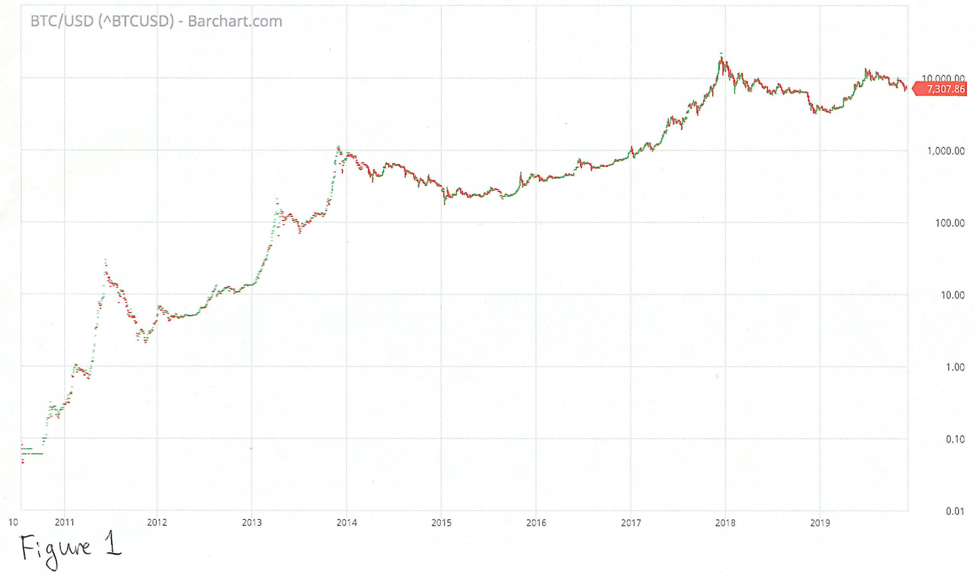
Fig. 1
I will use the chart with bars,located close to each other. This display fits the full BTC price range at each time point, so that we can determine if the waves overlap (this is important when calculating Elliott waves). I’ll have to draw the waves on the chart and put other marks by hand on paper, but it will be even more fun.
Finally, I will use the logarithmicthe scale. The step along the vertical axis, the price axis, will be degrees of ten (10, 100, 1000, etc.), and not linear (10, 20, 30, etc.). This choice is due to the fact that on a logarithmic scale, price movements appear in a more relevant form for investors, and our thesis is that price fluctuations are due to the mass psychology of investors.
I will give an example. Let's say you bought bitcoins for $ 100 when they cost $ 1 per bitcoin. ~ That is, you have acquired 100 ₿. If you sold them for $ 18, you would receive $ 1800 (and you would be very unhappy with this today). Now let's move forward several years when the price of bitcoin rose to $ 1000. Again, you buy bitcoins for $ 100, but this time you get only 0.1 ₿ for this money. Selling them at a price of $ 18,000, you, again, get $ 1800.
Thus, the price movement from 1 to 18 dollarshas exactly the same meaning as the movement from 1000 to 18 000 dollars, because the investor can earn the same amount. On a logarithmic scale, these two price ranges are of equal size on the X scale, while on a line chart, movements up to $ 18 will be completely indistinguishable compared to rallies up to $ 18,000. With the width of the price ranges through which bitcoin has passed over the years, line charts are practically useless for our purposes.
If this is not yet clear enough, then the general trendBitcoin prices are up. Bitcoin started growing at around $ 0.06 at the end of 2010 and peaked at ~ $ 20,000 a couple of years ago. One of the features of Bitcoin is that we have a full history of its price.
This is especially useful in light of curves.Elliott. We have an absolute reference point, followed by a clear uptrend, so there is no question of context. What we see is not part of a larger picture, invisible to the eye. We have all 100% of the price information (except for the future price, of course).
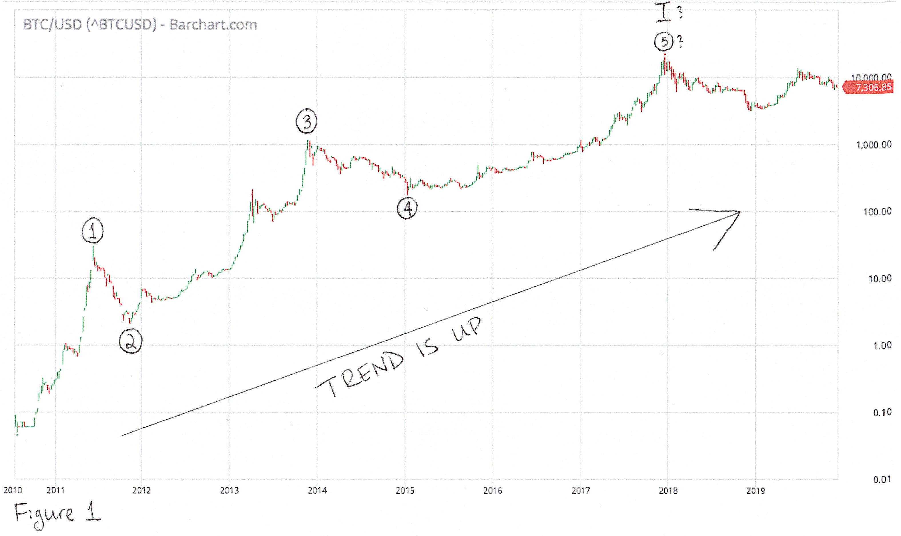
Fig. 2
This is a classic impulse movement consisting ofof the five waves that I labeled ①, ②, ③, ④ and ⑤ in Fig. 2. The circled numbers are the designation of Elliott waves of the primary level. The labeling and naming is arbitrary, but classical Elliott analysis typically uses this label for waves of this length. You may also notice the capital Roman numeral «I». This is the designation of the first wave of the main (cycle) level (one order of magnitude higher than the primary). I put question marks opposite ⑤ and I, because we are still unsure of the correct location of these marks. (I gave a brief explanation of the Elliott wave theory in a previous post).
Wave ①, the first primary ascending wave, clearlyis divided into five smaller waves nested within it, which is what we would expect from an impulse wave moving in the direction of a larger trend. These five «average» (intermediate) waves are designated in Figure 3 as (1), (2), (3), (4) and (5).
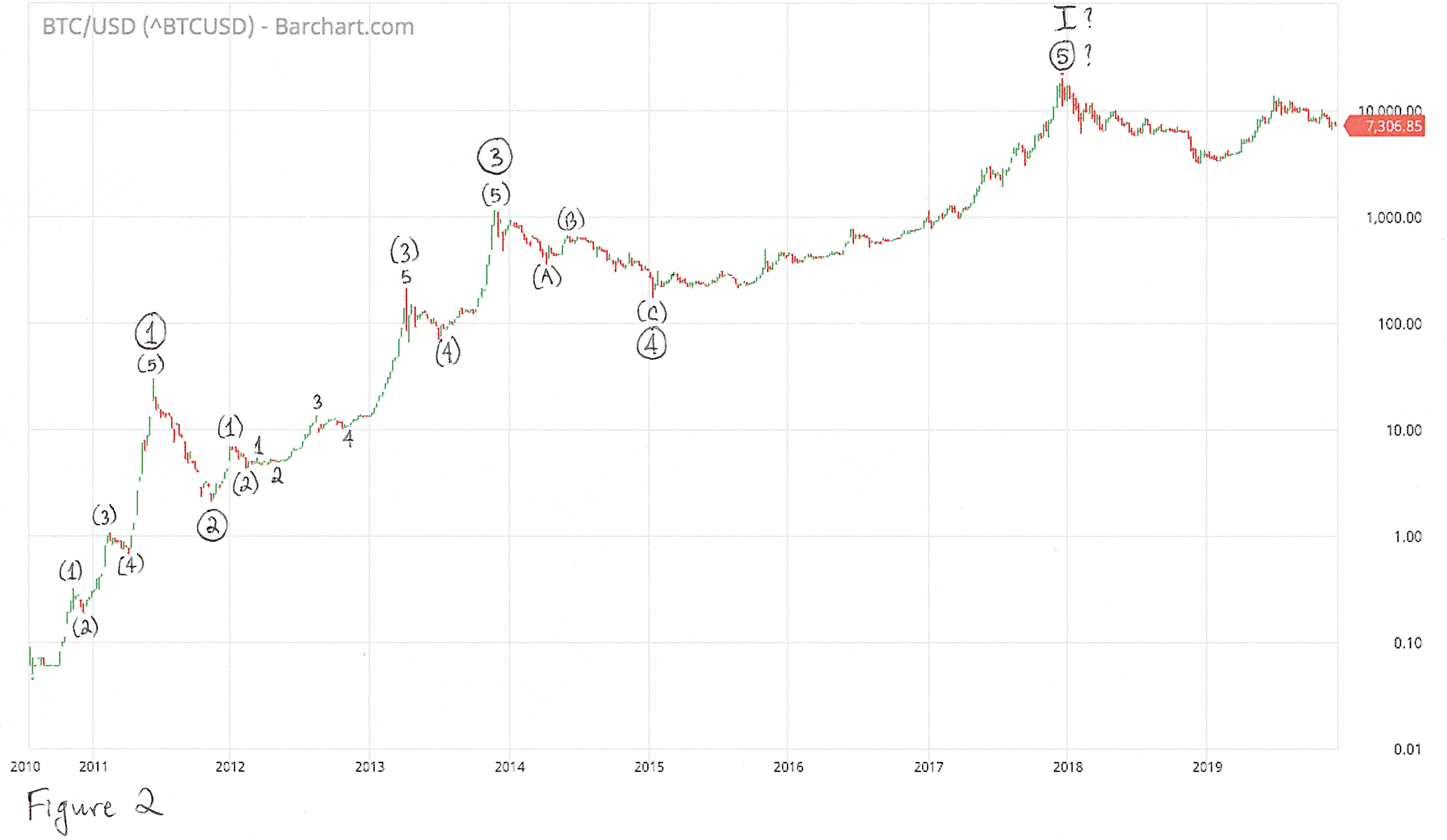
Fig. 3
The wave ② is corrective (it is directedagainst a larger trend). Its average subwaves are expressed implicitly (as is often the case with corrective waves), but overall this is a strong correction, amounting to more than 90% of the wave роста growth.
Wave ③ does not have such an obvious substructure,like wave ①, but is definitely impulsive. As a result, the price rose from single digits to more than $1,000. Its dynamic sub-waves also have an exponential form of impulse waves. The difficulty here is to determine where one middle subwave ends and the next one begins. The way we label them in Figure 3 is called an “extended third wave,” which is not uncommon since the 3rd wave is often the most powerful wave of an impulse. Compared to the (3) sub-wave, the middle sub-waves (1) and (2) of wave ③ look small. Some of the «small» (minor) subwaves (1, 2, 3, 4 and 5 in Fig. 3) waves (3) even exceed waves (1) and (2). This is fine. The first and second waves are often like this, because at the time of their formation the transition to impulse is not yet obvious, and therefore the market is still heavily influenced by hidden pessimism remaining after the previous correction.
Finally, let's look at the wave ④. This is a classic "zigzag" correction, consisting of three sub-waves, indicated by (A), (B) and (C) in Fig. 3.
Waves ① to ④ are complete, so the mainthe difficulty now lies in analyzing the wave ⑤ in the absence of complete confidence that it is complete. Counting waves on historical data is quite simple. To do this as they develop is much more difficult, but also much more profitable. The correct calculation, made before the end of the next wave, allows you to predict future prices. We will move on to this part in the next post.
and: 1, 2